library(tidyverse)Wrangling your data 🤠 Recitation Solutions
Week 4
Introduction
Today you are going to be practicing what you learned in the wrangling lesson. The more you practice modifying your data the easier it becomes. Remember, there are many ways to accomplish the same outcome. In the recitation solutions, I will show you a few different ways to answer the prompts and you can see how they differ, and use the ones that resonate with you.
Load data
To practice, we will be using some data I have extracted from Gapminder. I am linking to two files that you can download to your computer, and then read them in like we learned in class.
- Data on the happiness index for many countries for many years
- Data on the life expectancy for many countries for many years
# read in happiness data from your computer
# mine has the path below since i have a subfolder called data where
# the happiness data is living
happiness <- read_csv("data/hapiscore_whr.csv")
Rows: 163 Columns: 19
── Column specification ────────────────────────────────────────────────────────
Delimiter: ","
chr (1): country
dbl (18): 2005, 2006, 2007, 2008, 2009, 2010, 2011, 2012, 2013, 2014, 2015, ...
ℹ Use `spec()` to retrieve the full column specification for this data.
ℹ Specify the column types or set `show_col_types = FALSE` to quiet this message.# read in life expectancy data from your computer
life_expectancy <- read_csv("data/life_expectancy.csv")Rows: 195 Columns: 302
── Column specification ────────────────────────────────────────────────────────
Delimiter: ","
chr (1): country
dbl (301): 1800, 1801, 1802, 1803, 1804, 1805, 1806, 1807, 1808, 1809, 1810,...
ℹ Use `spec()` to retrieve the full column specification for this data.
ℹ Specify the column types or set `show_col_types = FALSE` to quiet this message.Explore your data
Write some code that lets you explore that is in these two datasets.
# see data structure with glimpse
glimpse(happiness)
Rows: 163
Columns: 19
$ country <chr> "Afghanistan", "Angola", "Albania", "United Arab Emirates", "A…
$ `2005` <dbl> NA, NA, NA, NA, NA, NA, 73.4, NA, NA, NA, 72.6, NA, NA, NA, NA…
$ `2006` <dbl> NA, NA, NA, 67.3, 63.1, 42.9, NA, 71.2, 47.3, NA, NA, 33.3, 38…
$ `2007` <dbl> NA, NA, 46.3, NA, 60.7, 48.8, 72.8, NA, 45.7, NA, 72.2, NA, 40…
$ `2008` <dbl> 37.2, NA, NA, NA, 59.6, 46.5, 72.5, 71.8, 48.2, 35.6, 71.2, 36…
$ `2009` <dbl> 44.0, NA, 54.9, 68.7, 64.2, 41.8, NA, NA, 45.7, 37.9, NA, NA, …
$ `2010` <dbl> 47.6, NA, 52.7, 71.0, 64.4, 43.7, 74.5, 73.0, 42.2, NA, 68.5, …
$ `2011` <dbl> 38.3, 55.9, 58.7, 71.2, 67.8, 42.6, 74.1, 74.7, 46.8, 37.1, 71…
$ `2012` <dbl> 37.8, 43.6, 55.1, 72.2, 64.7, 43.2, 72.0, 74.0, 49.1, NA, 69.3…
$ `2013` <dbl> 35.7, 39.4, 45.5, 66.2, 65.8, 42.8, 73.6, 75.0, 54.8, NA, 71.0…
$ `2014` <dbl> 31.3, 38.0, 48.1, 65.4, 66.7, 44.5, 72.9, 69.5, 52.5, 29.1, 68…
$ `2015` <dbl> 39.8, NA, 46.1, 65.7, 67.0, 43.5, 73.1, 70.8, 51.5, NA, 69.0, …
$ `2016` <dbl> 42.2, NA, 45.1, 68.3, 64.3, 43.3, 72.5, 70.5, 53.0, NA, 69.5, …
$ `2017` <dbl> 26.6, NA, 46.4, 70.4, 60.4, 42.9, 72.6, 72.9, 51.5, NA, 69.3, …
$ `2018` <dbl> 26.9, NA, 50.0, 66.0, 57.9, 50.6, 71.8, 74.0, 51.7, 37.8, 68.9…
$ `2019` <dbl> 23.8, NA, 50.0, 67.1, 60.9, 54.9, 72.3, 72.0, 51.7, NA, 67.7, …
$ `2020` <dbl> NA, NA, 53.6, 64.6, 59.0, NA, 71.4, 72.1, NA, NA, 68.4, 44.1, …
$ `2021` <dbl> 24.4, NA, 52.5, 67.3, 59.1, 53.0, 71.1, 70.8, NA, NA, 68.8, 44…
$ `2022` <dbl> 18.6, NA, 52.8, 65.7, 60.2, 53.4, 71.0, 71.0, NA, NA, 68.6, 43…# look at all columns and first 6 rows with head
head(happiness)# A tibble: 6 × 19
country `2005` `2006` `2007` `2008` `2009` `2010` `2011` `2012` `2013` `2014`
<chr> <dbl> <dbl> <dbl> <dbl> <dbl> <dbl> <dbl> <dbl> <dbl> <dbl>
1 Afghani… NA NA NA 37.2 44 47.6 38.3 37.8 35.7 31.3
2 Angola NA NA NA NA NA NA 55.9 43.6 39.4 38
3 Albania NA NA 46.3 NA 54.9 52.7 58.7 55.1 45.5 48.1
4 United … NA 67.3 NA NA 68.7 71 71.2 72.2 66.2 65.4
5 Argenti… NA 63.1 60.7 59.6 64.2 64.4 67.8 64.7 65.8 66.7
6 Armenia NA 42.9 48.8 46.5 41.8 43.7 42.6 43.2 42.8 44.5
# ℹ 8 more variables: `2015` <dbl>, `2016` <dbl>, `2017` <dbl>, `2018` <dbl>,
# `2019` <dbl>, `2020` <dbl>, `2021` <dbl>, `2022` <dbl># this will open the file for you to look through in R
# View(happiness)# see data structure with glimpse
glimpse(life_expectancy)Rows: 195
Columns: 302
$ country <chr> "Afghanistan", "Angola", "Albania", "Andorra", "United Arab Em…
$ `1800` <dbl> 28.2, 27.0, 35.4, NA, 30.7, 33.2, 34.0, 33.5, 34.0, 34.4, 29.2…
$ `1801` <dbl> 28.2, 27.0, 35.4, NA, 30.7, 33.2, 34.0, 33.5, 34.0, 34.4, 29.2…
$ `1802` <dbl> 28.2, 27.0, 35.4, NA, 30.7, 33.2, 34.0, 33.5, 34.0, 34.4, 29.2…
$ `1803` <dbl> 28.2, 27.0, 35.4, NA, 30.7, 33.2, 34.0, 33.5, 34.0, 34.4, 29.2…
$ `1804` <dbl> 28.2, 27.0, 35.4, NA, 30.7, 33.2, 34.0, 33.5, 34.0, 34.4, 29.2…
$ `1805` <dbl> 28.2, 27.0, 35.4, NA, 30.7, 33.2, 34.0, 33.5, 34.0, 34.4, 29.2…
$ `1806` <dbl> 28.1, 27.0, 35.4, NA, 30.7, 33.2, 34.0, 33.5, 34.0, 34.4, 29.2…
$ `1807` <dbl> 28.1, 27.0, 35.4, NA, 30.7, 33.2, 34.0, 33.5, 34.0, 34.4, 29.2…
$ `1808` <dbl> 28.1, 27.0, 35.4, NA, 30.7, 33.2, 34.0, 33.5, 34.0, 34.4, 29.2…
$ `1809` <dbl> 28.1, 27.0, 35.4, NA, 30.7, 33.2, 34.0, 33.5, 34.0, 34.4, 29.2…
$ `1810` <dbl> 28.1, 27.0, 35.4, NA, 30.7, 33.2, 34.0, 33.5, 34.0, 34.4, 29.2…
$ `1811` <dbl> 28.1, 27.0, 35.4, NA, 30.7, 33.2, 34.0, 33.5, 34.0, 34.4, 29.2…
$ `1812` <dbl> 28.1, 27.0, 35.4, NA, 30.7, 33.2, 34.0, 33.5, 34.0, 34.4, 29.2…
$ `1813` <dbl> 28.1, 27.0, 35.4, NA, 30.7, 33.2, 34.0, 33.5, 34.0, 34.4, 29.2…
$ `1814` <dbl> 28.1, 27.0, 35.4, NA, 30.7, 33.2, 34.0, 33.5, 34.0, 34.4, 29.2…
$ `1815` <dbl> 28.1, 27.0, 35.4, NA, 30.7, 33.2, 34.0, 33.5, 34.0, 34.4, 29.2…
$ `1816` <dbl> 28.1, 27.0, 35.4, NA, 30.7, 33.2, 34.0, 33.5, 34.0, 34.4, 29.2…
$ `1817` <dbl> 28.0, 27.0, 35.4, NA, 30.7, 33.2, 34.0, 33.5, 34.0, 34.4, 29.2…
$ `1818` <dbl> 28.0, 27.0, 35.4, NA, 30.7, 33.2, 34.0, 33.5, 34.0, 34.4, 29.2…
$ `1819` <dbl> 28.0, 27.0, 35.4, NA, 30.7, 33.2, 34.0, 33.5, 34.0, 34.4, 29.2…
$ `1820` <dbl> 28.0, 27.0, 35.4, NA, 30.7, 33.2, 34.0, 33.5, 34.0, 34.4, 29.2…
$ `1821` <dbl> 28.0, 27.0, 35.4, NA, 30.7, 33.2, 34.0, 33.5, 34.0, 34.4, 29.2…
$ `1822` <dbl> 28.0, 27.0, 35.4, NA, 30.7, 33.2, 34.0, 33.5, 34.0, 34.4, 29.2…
$ `1823` <dbl> 28.0, 27.0, 35.4, NA, 30.7, 33.2, 34.0, 33.5, 34.0, 34.4, 29.2…
$ `1824` <dbl> 28.0, 27.0, 35.4, NA, 30.7, 33.2, 34.0, 33.5, 34.0, 34.4, 29.2…
$ `1825` <dbl> 27.9, 27.0, 35.4, NA, 30.7, 33.2, 34.0, 33.5, 34.0, 34.4, 29.2…
$ `1826` <dbl> 27.9, 27.0, 35.4, NA, 30.7, 33.2, 34.0, 33.5, 34.0, 34.4, 29.2…
$ `1827` <dbl> 27.9, 27.0, 35.4, NA, 30.7, 33.2, 34.0, 33.5, 34.0, 34.4, 29.2…
$ `1828` <dbl> 27.9, 27.0, 35.4, NA, 30.7, 33.2, 34.0, 33.5, 34.0, 34.4, 29.2…
$ `1829` <dbl> 27.9, 27.0, 35.4, NA, 30.7, 33.2, 34.0, 33.5, 34.0, 34.4, 29.2…
$ `1830` <dbl> 27.9, 27.0, 35.4, NA, 30.7, 33.2, 34.0, 33.5, 34.0, 34.4, 29.2…
$ `1831` <dbl> 27.9, 27.0, 35.4, NA, 30.7, 33.2, 34.0, 33.5, 34.0, 34.4, 29.2…
$ `1832` <dbl> 27.9, 27.0, 35.4, NA, 30.7, 33.2, 34.0, 33.5, 34.0, 34.4, 29.2…
$ `1833` <dbl> 27.9, 27.0, 35.4, NA, 30.7, 33.2, 34.0, 33.5, 34.0, 34.4, 29.2…
$ `1834` <dbl> 27.9, 27.0, 35.4, NA, 30.7, 33.2, 34.0, 33.5, 34.0, 34.4, 29.2…
$ `1835` <dbl> 27.9, 27.0, 35.4, NA, 30.7, 33.2, 34.0, 33.5, 34.0, 34.4, 29.2…
$ `1836` <dbl> 27.8, 27.0, 35.4, NA, 30.7, 33.2, 34.0, 33.5, 34.0, 34.4, 29.2…
$ `1837` <dbl> 27.8, 27.0, 35.4, NA, 30.7, 33.2, 34.0, 33.5, 34.0, 34.4, 29.2…
$ `1838` <dbl> 27.8, 27.0, 35.4, NA, 30.7, 33.2, 34.0, 33.5, 34.0, 34.4, 29.2…
$ `1839` <dbl> 27.8, 27.0, 35.4, NA, 30.7, 33.2, 34.0, 33.5, 34.0, 34.4, 29.2…
$ `1840` <dbl> 27.8, 27.0, 35.4, NA, 30.7, 33.2, 34.0, 33.5, 34.0, 34.4, 29.2…
$ `1841` <dbl> 27.8, 27.0, 35.4, NA, 30.7, 33.2, 34.0, 33.5, 34.0, 34.4, 29.2…
$ `1842` <dbl> 27.8, 27.0, 35.4, NA, 30.7, 33.2, 34.0, 33.5, 34.0, 34.4, 29.2…
$ `1843` <dbl> 27.8, 27.0, 35.4, NA, 30.7, 33.2, 34.0, 33.5, 34.0, 34.4, 29.2…
$ `1844` <dbl> 27.8, 27.0, 35.4, NA, 30.7, 33.2, 34.0, 33.5, 34.0, 34.4, 29.2…
$ `1845` <dbl> 27.8, 27.0, 35.4, NA, 30.7, 33.2, 34.0, 33.5, 34.0, 34.4, 29.2…
$ `1846` <dbl> 27.7, 27.0, 35.4, NA, 30.7, 33.2, 34.0, 33.5, 34.0, 34.4, 29.2…
$ `1847` <dbl> 27.7, 27.0, 35.4, NA, 30.7, 33.2, 34.0, 33.5, 34.0, 34.4, 29.2…
$ `1848` <dbl> 27.7, 27.0, 35.4, NA, 30.7, 33.2, 34.0, 33.5, 34.0, 34.4, 29.2…
$ `1849` <dbl> 27.7, 27.0, 35.4, NA, 30.7, 33.2, 34.0, 33.5, 34.0, 34.4, 29.2…
$ `1850` <dbl> 27.7, 27.0, 35.4, NA, 30.7, 33.2, 34.0, 33.5, 34.0, 34.4, 29.2…
$ `1851` <dbl> 27.7, 27.0, 35.4, NA, 30.7, 33.2, 34.0, 33.5, 34.0, 34.4, 29.2…
$ `1852` <dbl> 27.7, 27.0, 35.4, NA, 30.7, 33.2, 34.0, 33.5, 34.0, 34.4, 29.2…
$ `1853` <dbl> 27.7, 27.0, 35.4, NA, 30.7, 33.2, 34.0, 33.5, 34.0, 34.4, 29.2…
$ `1854` <dbl> 27.7, 27.0, 35.4, NA, 30.7, 33.2, 34.0, 33.5, 34.0, 34.4, 29.2…
$ `1855` <dbl> 27.6, 27.0, 35.4, NA, 30.7, 33.2, 34.0, 33.5, 34.0, 34.4, 29.2…
$ `1856` <dbl> 27.6, 27.0, 35.4, NA, 30.7, 33.2, 34.0, 33.5, 34.0, 34.4, 29.2…
$ `1857` <dbl> 27.6, 27.0, 35.4, NA, 30.7, 33.2, 34.0, 33.5, 34.0, 34.4, 29.2…
$ `1858` <dbl> 27.6, 27.0, 35.4, NA, 30.7, 33.2, 34.0, 33.5, 34.0, 34.4, 29.2…
$ `1859` <dbl> 27.6, 27.0, 35.4, NA, 30.7, 33.2, 34.0, 33.5, 34.0, 34.4, 29.2…
$ `1860` <dbl> 27.6, 27.0, 35.4, NA, 30.7, 33.2, 34.0, 33.5, 34.0, 34.4, 29.2…
$ `1861` <dbl> 27.6, 27.0, 35.4, NA, 30.7, 33.2, 34.0, 33.5, 34.0, 34.4, 29.2…
$ `1862` <dbl> 27.6, 27.0, 35.4, NA, 30.7, 33.2, 34.0, 33.5, 34.0, 34.4, 29.2…
$ `1863` <dbl> 27.6, 27.0, 35.4, NA, 30.7, 33.2, 34.0, 33.5, 34.0, 34.4, 29.2…
$ `1864` <dbl> 27.6, 27.0, 35.4, NA, 30.7, 33.2, 33.5, 33.5, 34.0, 34.4, 28.6…
$ `1865` <dbl> 27.5, 27.0, 35.4, NA, 30.7, 33.2, 33.0, 33.5, 34.0, 34.4, 28.1…
$ `1866` <dbl> 27.5, 27.0, 35.4, NA, 30.7, 33.2, 32.4, 33.5, 34.0, 34.4, 27.6…
$ `1867` <dbl> 27.5, 27.0, 35.4, NA, 30.7, 33.2, 31.9, 33.5, 34.0, 34.4, 27.1…
$ `1868` <dbl> 27.5, 27.0, 35.4, NA, 30.7, 33.2, 31.4, 33.5, 34.0, 34.4, 26.6…
$ `1869` <dbl> 27.5, 27.0, 35.4, NA, 30.7, 33.2, 31.4, 33.5, 34.0, 34.4, 26.6…
$ `1870` <dbl> 27.5, 27.0, 35.4, NA, 30.7, 33.2, 31.5, 33.5, 34.0, 34.4, 26.6…
$ `1871` <dbl> 27.7, 27.2, 35.4, NA, 30.9, 33.2, 31.5, 33.5, 34.6, 34.5, 26.6…
$ `1872` <dbl> 27.9, 27.4, 35.4, NA, 31.0, 33.2, 31.6, 33.5, 35.1, 34.5, 26.5…
$ `1873` <dbl> 28.1, 27.6, 35.4, NA, 31.2, 33.2, 31.6, 33.5, 35.6, 34.6, 26.4…
$ `1874` <dbl> 28.3, 27.7, 35.3, NA, 31.3, 33.3, 31.8, 33.5, 36.2, 34.6, 26.5…
$ `1875` <dbl> 28.5, 27.9, 35.3, NA, 31.5, 33.3, 32.0, 33.6, 36.7, 34.7, 26.6…
$ `1876` <dbl> 28.7, 28.1, 35.3, NA, 31.6, 33.3, 32.2, 33.6, 37.2, 34.7, 26.7…
$ `1877` <dbl> 28.9, 28.3, 35.3, NA, 31.8, 33.3, 32.4, 33.6, 37.8, 34.8, 26.8…
$ `1878` <dbl> 29.1, 28.5, 35.3, NA, 32.0, 33.2, 32.6, 33.6, 38.3, 34.8, 26.8…
$ `1879` <dbl> 29.3, 28.7, 35.3, NA, 32.1, 33.2, 32.8, 33.6, 38.8, 34.9, 26.9…
$ `1880` <dbl> 29.4, 28.9, 35.2, NA, 32.3, 33.2, 33.0, 33.6, 39.4, 34.9, 27.0…
$ `1881` <dbl> 29.6, 29.1, 35.2, NA, 32.4, 33.1, 33.2, 33.6, 39.9, 35.0, 27.0…
$ `1882` <dbl> 29.8, 29.3, 35.2, NA, 32.6, 33.0, 33.4, 33.6, 40.4, 35.2, 27.1…
$ `1883` <dbl> 30.0, 29.4, 35.2, NA, 32.8, 33.0, 33.6, 33.6, 41.0, 35.5, 27.2…
$ `1884` <dbl> 30.2, 29.6, 35.2, NA, 32.9, 32.9, 33.8, 33.6, 41.5, 35.7, 27.3…
$ `1885` <dbl> 30.4, 29.8, 35.2, NA, 33.1, 32.8, 34.0, 33.6, 42.0, 35.9, 27.3…
$ `1886` <dbl> 30.6, 30.0, 35.1, NA, 33.2, 33.1, 34.2, 33.6, 42.6, 36.1, 27.4…
$ `1887` <dbl> 30.8, 30.2, 35.1, NA, 33.4, 33.4, 34.4, 33.6, 43.1, 36.4, 27.4…
$ `1888` <dbl> 31.0, 30.4, 35.1, NA, 33.5, 33.7, 34.6, 33.6, 43.6, 36.6, 27.5…
$ `1889` <dbl> 31.2, 30.6, 35.1, NA, 33.7, 34.0, 34.8, 33.6, 44.2, 36.8, 27.6…
$ `1890` <dbl> 31.4, 30.8, 35.1, NA, 33.9, 34.3, 35.0, 33.6, 44.7, 37.1, 27.6…
$ `1891` <dbl> 31.6, 30.9, 35.1, NA, 34.0, 34.1, 35.2, 33.6, 45.2, 37.3, 27.7…
$ `1892` <dbl> 31.8, 31.1, 35.0, NA, 34.2, 34.0, 35.4, 33.6, 45.8, 37.8, 27.7…
$ `1893` <dbl> 32.0, 31.3, 35.0, NA, 34.3, 33.9, 35.6, 33.6, 46.3, 38.2, 27.8…
$ `1894` <dbl> 32.2, 31.5, 35.0, NA, 34.5, 33.8, 35.8, 33.6, 46.8, 38.7, 27.8…
$ `1895` <dbl> 32.4, 31.7, 35.0, NA, 34.6, 33.6, 36.0, 33.6, 47.4, 39.2, 27.9…
$ `1896` <dbl> 32.5, 31.9, 35.0, NA, 34.8, 34.3, 36.2, 33.6, 47.9, 39.6, 27.9…
$ `1897` <dbl> 32.7, 32.1, 35.0, NA, 35.0, 35.1, 36.4, 33.6, 48.4, 40.1, 28.0…
$ `1898` <dbl> 32.9, 32.3, 35.0, NA, 35.1, 35.8, 36.2, 33.7, 49.0, 40.6, 27.7…
$ `1899` <dbl> 33.1, 32.5, 34.9, NA, 35.3, 36.5, 36.1, 33.7, 49.5, 41.0, 27.4…
$ `1900` <dbl> 33.3, 32.6, 34.9, NA, 35.4, 37.2, 35.9, 33.7, 50.0, 41.5, 27.1…
$ `1901` <dbl> 33.5, 32.8, 34.9, NA, 35.6, 37.8, 36.1, 33.7, 50.6, 42.0, 27.2…
$ `1902` <dbl> 33.7, 33.0, 34.9, NA, 35.7, 38.4, 36.4, 33.7, 51.1, 41.0, 27.3…
$ `1903` <dbl> 33.9, 33.2, 34.9, NA, 35.9, 39.0, 36.6, 33.7, 51.6, 40.1, 27.4…
$ `1904` <dbl> 34.1, 33.4, 34.9, NA, 36.1, 39.6, 36.9, 33.7, 52.2, 40.7, 27.4…
$ `1905` <dbl> 34.3, 33.6, 34.8, NA, 36.2, 40.2, 37.1, 33.7, 52.7, 41.3, 27.5…
$ `1906` <dbl> 34.5, 33.8, 34.8, NA, 36.4, 41.0, 37.4, 33.7, 53.2, 42.0, 27.6…
$ `1907` <dbl> 34.7, 34.0, 34.8, NA, 36.5, 41.8, 37.6, 33.7, 53.8, 42.6, 27.7…
$ `1908` <dbl> 34.9, 34.2, 34.8, NA, 36.7, 42.6, 37.9, 33.7, 54.3, 43.2, 27.8…
$ `1909` <dbl> 35.0, 34.4, 34.8, NA, 36.8, 43.4, 38.1, 33.7, 54.8, 43.8, 27.8…
$ `1910` <dbl> 35.2, 34.5, 34.8, NA, 37.0, 44.2, 38.4, 33.7, 55.4, 44.5, 27.9…
$ `1911` <dbl> 35.4, 34.7, 34.7, NA, 37.2, 44.7, 41.4, 33.7, 55.9, 45.1, 30.2…
$ `1912` <dbl> 35.6, 34.9, 34.7, NA, 37.3, 45.3, 41.8, 33.7, 56.4, 45.6, 30.4…
$ `1913` <dbl> 35.8, 35.1, 34.7, NA, 37.5, 45.9, 39.6, 33.7, 57.0, 46.2, 28.4…
$ `1914` <dbl> 36.0, 35.3, 34.7, NA, 37.6, 46.4, 39.2, 33.7, 57.5, 46.8, 28.0…
$ `1915` <dbl> 36.2, 35.5, 34.7, NA, 37.8, 47.0, 38.8, 33.7, 58.0, 47.3, 27.5…
$ `1916` <dbl> 36.4, 35.7, 34.7, NA, 38.0, 47.8, 38.8, 33.7, 58.6, 47.9, 27.4…
$ `1917` <dbl> 36.6, 35.9, 34.6, NA, 38.1, 48.7, 35.8, 33.7, 59.1, 48.5, 24.8…
$ `1918` <dbl> 9.59, 13.90, 19.00, NA, 31.70, 42.50, 27.00, 21.90, 55.00, 32.…
$ `1919` <dbl> 36.9, 36.2, 34.6, NA, 38.4, 50.3, 37.0, 33.8, 60.2, 49.6, 25.4…
$ `1920` <dbl> 37.1, 36.4, 34.6, NA, 38.6, 51.2, 28.0, 33.8, 60.7, 50.2, 23.6…
$ `1921` <dbl> 37.3, 36.6, 34.6, NA, 38.7, 51.7, 38.0, 33.8, 61.3, 50.7, 25.9…
$ `1922` <dbl> 37.5, 36.8, 34.6, NA, 38.9, 52.2, 39.0, 34.6, 63.1, 51.3, 26.5…
$ `1923` <dbl> 37.7, 37.0, 34.5, NA, 39.0, 52.7, 39.9, 35.4, 62.0, 51.9, 27.2…
$ `1924` <dbl> 37.9, 37.2, 34.5, NA, 39.2, 53.2, 42.4, 36.3, 62.8, 52.4, 29.0…
$ `1925` <dbl> 38.1, 37.4, 34.5, NA, 39.4, 53.7, 41.5, 37.1, 63.5, 53.0, 28.1…
$ `1926` <dbl> 38.3, 37.6, 34.5, NA, 39.5, 54.1, 44.7, 38.0, 63.2, 53.6, 30.4…
$ `1927` <dbl> 38.4, 37.8, 34.5, NA, 39.7, 54.4, 44.0, 38.8, 63.2, 54.1, 29.7…
$ `1928` <dbl> 38.6, 37.9, 34.5, NA, 39.8, 54.8, 45.5, 39.6, 63.2, 54.7, 30.7…
$ `1929` <dbl> 38.8, 38.1, 34.5, NA, 40.0, 55.2, 44.3, 40.5, 63.4, 55.3, 29.6…
$ `1930` <dbl> 39.0, 38.3, 35.3, NA, 40.1, 55.5, 43.6, 41.3, 65.2, 55.8, 28.9…
$ `1931` <dbl> 39.2, 38.5, 36.1, NA, 40.3, 55.6, 42.0, 42.1, 65.7, 56.4, 27.4…
$ `1932` <dbl> 39.4, 38.7, 37.0, NA, 40.5, 55.6, 39.5, 43.0, 66.0, 56.7, 25.4…
$ `1933` <dbl> 39.6, 38.9, 37.9, NA, 40.6, 55.6, 33.0, 43.8, 65.8, 57.0, 19.8…
$ `1934` <dbl> 39.8, 39.1, 38.7, NA, 40.8, 55.6, 46.0, 44.7, 65.2, 57.3, 30.0…
$ `1935` <dbl> 39.9, 39.3, 39.6, NA, 40.9, 55.6, 47.5, 45.5, 65.4, 57.6, 30.9…
$ `1936` <dbl> 40.1, 39.5, 40.4, NA, 41.1, 56.6, 49.2, 46.3, 65.6, 57.9, 32.0…
$ `1937` <dbl> 40.3, 39.6, 41.3, NA, 41.3, 57.7, 48.2, 47.2, 66.1, 58.2, 31.1…
$ `1938` <dbl> 40.5, 39.8, 42.1, NA, 41.4, 58.7, 49.9, 48.0, 66.2, 58.5, 32.1…
$ `1939` <dbl> 40.7, 40.0, 41.6, NA, 41.6, 59.7, 52.3, 48.9, 66.1, 58.0, 33.6…
$ `1940` <dbl> 40.9, 40.2, 40.7, NA, 41.7, 60.7, 49.8, 49.7, 66.6, 57.7, 31.6…
$ `1941` <dbl> 41.0, 40.7, 40.1, NA, 41.9, 61.3, 27.4, 50.5, 66.5, 56.4, 21.2…
$ `1942` <dbl> 41.2, 41.3, 38.7, NA, 42.0, 61.9, 23.5, 51.4, 66.2, 54.0, 18.6…
$ `1943` <dbl> 41.4, 41.8, 35.8, NA, 42.2, 62.5, 21.1, 52.2, 66.7, 50.1, 17.1…
$ `1944` <dbl> 41.6, 42.3, 32.9, NA, 42.4, 63.2, 27.5, 53.1, 68.4, 39.1, 22.0…
$ `1945` <dbl> 41.8, 42.9, 45.4, NA, 42.5, 63.8, 35.4, 53.9, 68.8, 31.4, 28.7…
$ `1946` <dbl> 42.0, 43.4, 48.3, NA, 45.6, 63.7, 49.6, 54.8, 68.3, 55.9, 35.3…
$ `1947` <dbl> 42.2, 43.9, 49.7, NA, 48.8, 63.6, 41.5, 55.6, 69.0, 61.2, 29.6…
$ `1948` <dbl> 42.4, 44.5, 50.5, NA, 52.0, 63.5, 47.0, 56.5, 68.9, 63.2, 34.9…
$ `1949` <dbl> 42.5, 45.0, 51.4, NA, 55.2, 63.4, 47.9, 57.3, 69.5, 63.4, 36.5…
$ `1950` <dbl> 42.7, 45.6, 52.2, 74.6, 58.4, 63.3, 48.2, 58.1, 69.4, 64.8, 37…
$ `1951` <dbl> 42.9, 45.6, 53.6, 74.7, 58.5, 63.5, 49.0, 58.7, 69.2, 65.5, 38…
$ `1952` <dbl> 43.1, 45.6, 54.5, 74.8, 58.6, 64.2, 50.0, 59.3, 69.5, 66.7, 39…
$ `1953` <dbl> 43.5, 45.6, 55.4, 75.0, 58.7, 64.1, 51.1, 59.8, 69.9, 67.2, 40…
$ `1954` <dbl> 43.3, 45.6, 56.1, 75.1, 58.8, 64.7, 52.1, 60.3, 70.2, 67.3, 41…
$ `1955` <dbl> 43.9, 45.5, 56.3, 75.2, 58.9, 64.5, 53.3, 60.9, 70.3, 67.7, 42…
$ `1956` <dbl> 44.1, 45.7, 58.0, 75.3, 58.8, 65.2, 54.5, 61.5, 70.4, 67.8, 43…
$ `1957` <dbl> 44.3, 45.8, 59.3, 75.4, 59.3, 65.2, 55.7, 61.9, 70.6, 67.8, 44…
$ `1958` <dbl> 44.5, 45.9, 61.0, 75.5, 59.6, 65.4, 56.5, 62.6, 71.0, 68.4, 45…
$ `1959` <dbl> 44.7, 46.1, 61.7, 75.6, 59.7, 65.4, 58.0, 63.3, 70.9, 68.5, 46…
$ `1960` <dbl> 45.0, 46.3, 62.5, 75.7, 60.3, 65.3, 59.2, 63.8, 71.1, 69.0, 48…
$ `1961` <dbl> 45.3, 44.8, 63.3, 75.8, 60.8, 65.7, 60.4, 64.8, 71.3, 69.6, 50…
$ `1962` <dbl> 45.5, 45.0, 63.3, 75.9, 61.3, 65.8, 61.4, 65.5, 71.2, 69.7, 51…
$ `1963` <dbl> 45.7, 45.2, 63.8, 76.0, 61.6, 65.8, 62.0, 65.8, 71.2, 69.8, 53…
$ `1964` <dbl> 45.9, 45.4, 64.4, 76.2, 62.1, 65.8, 62.9, 66.1, 71.0, 70.0, 54…
$ `1965` <dbl> 46.1, 45.6, 64.8, 76.3, 62.6, 66.1, 63.6, 66.7, 71.1, 70.1, 55…
$ `1966` <dbl> 46.3, 45.8, 65.5, 76.4, 63.0, 66.6, 64.2, 67.1, 71.1, 70.2, 56…
$ `1967` <dbl> 46.5, 46.0, 66.1, 76.5, 63.4, 66.5, 64.7, 67.2, 71.1, 70.2, 57…
$ `1968` <dbl> 46.7, 46.2, 66.5, 76.7, 63.8, 66.0, 65.1, 67.6, 71.0, 70.3, 58…
$ `1969` <dbl> 46.9, 46.4, 67.1, 76.8, 64.2, 65.9, 65.3, 68.0, 71.2, 70.2, 58…
$ `1970` <dbl> 47.1, 46.6, 67.8, 77.0, 64.0, 66.1, 65.9, 68.3, 71.2, 70.2, 59…
$ `1971` <dbl> 47.3, 46.8, 68.3, 77.1, 64.9, 66.9, 66.4, 68.9, 71.4, 70.4, 61…
$ `1972` <dbl> 47.3, 47.0, 68.8, 77.2, 65.1, 67.3, 66.8, 69.4, 71.8, 70.7, 61…
$ `1973` <dbl> 47.3, 47.2, 69.3, 77.4, 65.4, 67.7, 67.2, 69.8, 71.9, 71.1, 62…
$ `1974` <dbl> 47.4, 47.4, 69.8, 77.5, 65.7, 67.9, 67.9, 70.0, 72.0, 71.2, 63…
$ `1975` <dbl> 47.5, 47.5, 70.2, 77.7, 66.0, 68.0, 68.2, 70.2, 72.5, 71.4, 64…
$ `1976` <dbl> 47.7, 47.5, 70.7, 77.8, 66.3, 67.0, 69.0, 70.3, 72.8, 71.8, 65…
$ `1977` <dbl> 47.9, 47.7, 71.1, 78.0, 66.6, 67.7, 69.5, 70.6, 73.3, 72.2, 65…
$ `1978` <dbl> 46.4, 47.8, 71.7, 78.1, 67.0, 69.0, 69.7, 71.0, 73.8, 72.4, 64…
$ `1979` <dbl> 44.7, 48.0, 71.3, 78.2, 67.3, 69.8, 70.2, 71.6, 74.2, 72.6, 65…
$ `1980` <dbl> 43.7, 48.1, 71.3, 78.3, 67.6, 70.2, 70.2, 72.1, 74.5, 72.8, 66…
$ `1981` <dbl> 44.3, 48.2, 71.3, 78.4, 68.0, 70.3, 70.5, 72.6, 74.8, 73.1, 66…
$ `1982` <dbl> 44.1, 48.2, 71.4, 78.5, 68.1, 70.9, 70.8, 73.2, 74.9, 73.3, 66…
$ `1983` <dbl> 42.3, 48.2, 71.2, 78.5, 67.9, 70.7, 70.8, 73.8, 75.3, 73.5, 66…
$ `1984` <dbl> 39.9, 48.4, 71.4, 78.6, 68.4, 70.8, 71.1, 73.5, 75.5, 73.9, 66…
$ `1985` <dbl> 42.0, 48.6, 71.9, 78.7, 68.5, 71.7, 71.3, 73.8, 75.6, 74.3, 66…
$ `1986` <dbl> 43.3, 48.6, 72.3, 78.8, 68.5, 72.0, 71.7, 74.0, 76.0, 74.7, 66…
$ `1987` <dbl> 45.9, 48.6, 72.2, 78.8, 68.5, 72.1, 71.8, 74.2, 76.2, 75.1, 66…
$ `1988` <dbl> 48.5, 48.6, 72.4, 78.9, 68.5, 72.1, 55.3, 74.3, 76.4, 75.5, 66…
$ `1989` <dbl> 52.7, 49.4, 72.5, 79.0, 68.6, 72.3, 71.0, 74.3, 76.5, 75.7, 67…
$ `1990` <dbl> 53.8, 49.7, 72.8, 79.0, 68.7, 72.5, 70.6, 74.0, 77.0, 76.0, 66…
$ `1991` <dbl> 53.8, 50.3, 72.6, 79.1, 68.7, 72.7, 70.3, 74.0, 77.4, 76.1, 66…
$ `1992` <dbl> 54.2, 50.3, 73.2, 79.2, 68.8, 72.8, 69.4, 74.0, 77.6, 76.3, 64…
$ `1993` <dbl> 54.4, 49.0, 73.8, 79.3, 68.8, 73.0, 69.0, 73.4, 77.9, 76.5, 64…
$ `1994` <dbl> 53.9, 50.3, 74.6, 79.5, 68.7, 73.4, 69.5, 73.3, 78.0, 76.7, 63…
$ `1995` <dbl> 54.3, 51.2, 74.6, 79.8, 68.8, 73.4, 70.1, 73.3, 78.3, 77.0, 64…
$ `1996` <dbl> 54.7, 51.7, 74.5, 80.0, 68.9, 73.5, 70.4, 74.0, 78.5, 77.3, 65…
$ `1997` <dbl> 54.5, 51.6, 72.9, 80.2, 69.0, 73.6, 71.1, 73.5, 78.8, 77.7, 65…
$ `1998` <dbl> 53.3, 50.6, 74.8, 80.4, 69.2, 73.7, 71.6, 74.5, 79.1, 77.9, 66…
$ `1999` <dbl> 54.7, 51.9, 75.1, 80.6, 69.2, 73.8, 71.9, 74.7, 79.4, 78.2, 66…
$ `2000` <dbl> 54.7, 52.8, 75.4, 80.8, 69.1, 74.2, 72.4, 74.8, 79.7, 78.5, 66…
$ `2001` <dbl> 54.8, 53.4, 76.0, 80.9, 69.2, 74.3, 72.5, 75.1, 80.1, 78.9, 67…
$ `2002` <dbl> 55.5, 54.5, 75.9, 81.1, 69.4, 74.3, 72.7, 75.4, 80.3, 79.0, 67…
$ `2003` <dbl> 56.5, 55.1, 75.6, 81.2, 69.3, 74.4, 72.8, 75.6, 80.6, 79.1, 67…
$ `2004` <dbl> 57.1, 55.5, 75.8, 81.3, 69.1, 74.9, 73.0, 75.7, 80.9, 79.5, 67…
$ `2005` <dbl> 57.6, 56.4, 76.2, 81.4, 69.2, 75.3, 73.0, 75.9, 81.2, 79.8, 67…
$ `2006` <dbl> 58.0, 57.0, 76.9, 81.5, 69.5, 75.4, 73.1, 75.9, 81.5, 80.1, 67…
$ `2007` <dbl> 58.5, 58.0, 77.5, 81.7, 70.0, 75.3, 73.5, 75.1, 81.5, 80.3, 68…
$ `2008` <dbl> 59.2, 58.8, 77.6, 81.8, 70.4, 75.7, 73.5, 75.2, 81.7, 80.5, 68…
$ `2009` <dbl> 59.9, 59.5, 78.0, 81.8, 70.6, 75.8, 73.6, 75.8, 81.9, 80.5, 68…
$ `2010` <dbl> 60.5, 60.2, 78.1, 81.8, 70.8, 75.9, 73.9, 75.9, 82.1, 80.8, 69…
$ `2011` <dbl> 61.0, 60.8, 78.1, 81.9, 71.0, 76.0, 74.2, 76.0, 82.3, 81.0, 69…
$ `2012` <dbl> 61.4, 61.4, 78.2, 81.9, 71.2, 76.2, 74.6, 76.0, 82.6, 81.2, 69…
$ `2013` <dbl> 61.9, 62.1, 78.3, 82.0, 71.6, 76.3, 75.1, 76.1, 82.7, 81.3, 69…
$ `2014` <dbl> 61.9, 63.0, 78.2, 82.0, 73.0, 76.5, 75.2, 76.0, 82.7, 81.5, 69…
$ `2015` <dbl> 61.9, 63.5, 78.1, 82.0, 73.2, 76.5, 75.1, 76.0, 82.7, 81.6, 70…
$ `2016` <dbl> 62.0, 63.9, 78.2, 82.1, 73.4, 76.2, 75.3, 76.0, 83.0, 81.8, 70…
$ `2017` <dbl> 62.9, 64.2, 78.3, 82.1, 73.5, 76.3, 75.5, 76.1, 83.0, 82.0, 70…
$ `2018` <dbl> 62.7, 64.6, 78.4, 82.1, 73.7, 76.5, 75.6, 76.2, 82.9, 82.1, 70…
$ `2019` <dbl> 63.3, 65.1, 78.5, 82.2, 73.9, 76.6, 75.7, 76.3, 82.9, 82.2, 71…
$ `2020` <dbl> 63.4, 65.2, 77.9, NA, 74.0, 74.6, 74.0, 76.3, 82.9, 81.5, 70.4…
$ `2021` <dbl> 64.0, 65.8, 78.7, NA, 74.2, 76.9, 76.0, 76.5, 83.2, 82.4, 71.2…
$ `2022` <dbl> 64.3, 66.1, 78.8, NA, 74.3, 77.0, 76.1, 76.7, 83.3, 82.6, 71.3…
$ `2023` <dbl> 64.6, 66.4, 79.0, NA, 74.4, 77.2, 76.3, 76.8, 83.5, 82.8, 71.4…
$ `2024` <dbl> 64.9, 66.8, 79.1, NA, 74.6, 77.3, 76.4, 76.9, 83.6, 82.9, 71.5…
$ `2025` <dbl> 65.2, 67.1, 79.2, NA, 74.7, 77.5, 76.5, 77.1, 83.7, 83.1, 71.6…
$ `2026` <dbl> 65.4, 67.4, 79.4, NA, 74.8, 77.6, 76.7, 77.2, 83.8, 83.2, 71.7…
$ `2027` <dbl> 65.7, 67.7, 79.5, NA, 75.0, 77.8, 76.8, 77.3, 84.0, 83.4, 71.8…
$ `2028` <dbl> 66.0, 68.0, 79.7, NA, 75.1, 77.9, 77.0, 77.4, 84.1, 83.6, 71.9…
$ `2029` <dbl> 66.2, 68.3, 79.8, NA, 75.2, 78.0, 77.1, 77.6, 84.2, 83.7, 72.0…
$ `2030` <dbl> 66.4, 68.6, 80.0, NA, 75.4, 78.2, 77.2, 77.7, 84.3, 83.9, 72.1…
$ `2031` <dbl> 66.6, 68.9, 80.2, NA, 75.5, 78.3, 77.4, 77.8, 84.4, 84.1, 72.2…
$ `2032` <dbl> 66.9, 69.2, 80.3, NA, 75.6, 78.5, 77.5, 78.0, 84.6, 84.2, 72.3…
$ `2033` <dbl> 67.1, 69.4, 80.5, NA, 75.8, 78.6, 77.7, 78.1, 84.7, 84.4, 72.4…
$ `2034` <dbl> 67.3, 69.7, 80.7, NA, 75.9, 78.8, 77.8, 78.2, 84.8, 84.5, 72.5…
$ `2035` <dbl> 67.5, 70.0, 80.8, NA, 76.0, 78.9, 77.9, 78.3, 84.9, 84.7, 72.7…
$ `2036` <dbl> 67.7, 70.2, 80.9, NA, 76.2, 79.1, 78.1, 78.5, 85.0, 84.8, 72.8…
$ `2037` <dbl> 67.9, 70.5, 81.1, NA, 76.3, 79.2, 78.2, 78.6, 85.2, 84.9, 72.9…
$ `2038` <dbl> 68.0, 70.7, 81.2, NA, 76.4, 79.4, 78.3, 78.7, 85.3, 85.0, 73.0…
$ `2039` <dbl> 68.2, 70.9, 81.3, NA, 76.6, 79.5, 78.5, 78.8, 85.4, 85.2, 73.1…
$ `2040` <dbl> 68.4, 71.1, 81.5, NA, 76.7, 79.7, 78.6, 79.0, 85.5, 85.3, 73.2…
$ `2041` <dbl> 68.6, 71.4, 81.6, NA, 76.8, 79.8, 78.7, 79.1, 85.6, 85.4, 73.3…
$ `2042` <dbl> 68.8, 71.6, 81.8, NA, 77.0, 80.0, 78.9, 79.2, 85.7, 85.5, 73.5…
$ `2043` <dbl> 68.9, 71.8, 81.9, NA, 77.1, 80.1, 79.0, 79.3, 85.8, 85.6, 73.6…
$ `2044` <dbl> 69.1, 72.0, 82.0, NA, 77.2, 80.3, 79.1, 79.5, 86.0, 85.8, 73.7…
$ `2045` <dbl> 69.2, 72.2, 82.2, NA, 77.3, 80.4, 79.3, 79.6, 86.1, 85.9, 73.8…
$ `2046` <dbl> 69.4, 72.4, 82.3, NA, 77.5, 80.6, 79.4, 79.7, 86.2, 86.0, 73.9…
$ `2047` <dbl> 69.5, 72.5, 82.4, NA, 77.6, 80.7, 79.5, 79.8, 86.3, 86.1, 74.0…
$ `2048` <dbl> 69.7, 72.7, 82.6, NA, 77.7, 80.8, 79.7, 80.0, 86.4, 86.2, 74.2…
$ `2049` <dbl> 69.8, 72.9, 82.7, NA, 77.9, 81.0, 79.8, 80.1, 86.5, 86.3, 74.3…
$ `2050` <dbl> 70.0, 73.1, 82.8, NA, 78.0, 81.2, 79.9, 80.2, 86.6, 86.5, 74.4…
$ `2051` <dbl> 70.2, 73.3, 83.0, NA, 78.1, 81.3, 80.0, 80.3, 86.8, 86.6, 74.5…
$ `2052` <dbl> 70.3, 73.4, 83.1, NA, 78.2, 81.4, 80.2, 80.5, 86.9, 86.7, 74.6…
$ `2053` <dbl> 70.4, 73.6, 83.3, NA, 78.4, 81.6, 80.3, 80.6, 87.0, 86.8, 74.7…
$ `2054` <dbl> 70.6, 73.8, 83.4, NA, 78.5, 81.7, 80.5, 80.7, 87.1, 86.9, 74.9…
$ `2055` <dbl> 70.7, 73.9, 83.5, NA, 78.6, 81.9, 80.6, 80.8, 87.2, 87.0, 75.0…
$ `2056` <dbl> 70.9, 74.1, 83.7, NA, 78.7, 82.0, 80.7, 81.0, 87.3, 87.1, 75.1…
$ `2057` <dbl> 71.0, 74.2, 83.8, NA, 78.8, 82.2, 80.9, 81.1, 87.4, 87.3, 75.2…
$ `2058` <dbl> 71.1, 74.4, 83.9, NA, 79.0, 82.3, 81.0, 81.2, 87.5, 87.4, 75.3…
$ `2059` <dbl> 71.3, 74.5, 84.0, NA, 79.1, 82.4, 81.1, 81.3, 87.7, 87.5, 75.5…
$ `2060` <dbl> 71.4, 74.7, 84.1, NA, 79.2, 82.6, 81.3, 81.5, 87.8, 87.6, 75.6…
$ `2061` <dbl> 71.5, 74.8, 84.3, NA, 79.3, 82.7, 81.4, 81.6, 87.9, 87.7, 75.7…
$ `2062` <dbl> 71.7, 75.0, 84.4, NA, 79.4, 82.8, 81.5, 81.7, 88.0, 87.8, 75.8…
$ `2063` <dbl> 71.8, 75.1, 84.5, NA, 79.5, 83.0, 81.7, 81.8, 88.1, 87.9, 75.9…
$ `2064` <dbl> 72.0, 75.3, 84.6, NA, 79.7, 83.1, 81.8, 82.0, 88.2, 88.0, 76.1…
$ `2065` <dbl> 72.1, 75.4, 84.7, NA, 79.8, 83.2, 81.9, 82.1, 88.3, 88.1, 76.2…
$ `2066` <dbl> 72.2, 75.5, 84.8, NA, 79.9, 83.4, 82.1, 82.2, 88.5, 88.3, 76.3…
$ `2067` <dbl> 72.3, 75.7, 84.9, NA, 80.0, 83.5, 82.2, 82.3, 88.6, 88.4, 76.4…
$ `2068` <dbl> 72.5, 75.8, 85.0, NA, 80.1, 83.6, 82.3, 82.5, 88.7, 88.5, 76.6…
$ `2069` <dbl> 72.6, 76.0, 85.2, NA, 80.2, 83.7, 82.5, 82.6, 88.8, 88.6, 76.7…
$ `2070` <dbl> 72.7, 76.1, 85.3, NA, 80.3, 83.9, 82.6, 82.7, 88.9, 88.7, 76.8…
$ `2071` <dbl> 72.9, 76.2, 85.4, NA, 80.4, 84.0, 82.7, 82.8, 89.0, 88.8, 76.9…
$ `2072` <dbl> 73.0, 76.4, 85.5, NA, 80.5, 84.1, 82.9, 82.9, 89.1, 88.9, 77.1…
$ `2073` <dbl> 73.1, 76.5, 85.6, NA, 80.7, 84.2, 83.0, 83.0, 89.2, 89.0, 77.2…
$ `2074` <dbl> 73.3, 76.6, 85.7, NA, 80.8, 84.3, 83.1, 83.2, 89.3, 89.1, 77.3…
$ `2075` <dbl> 73.4, 76.8, 85.8, NA, 80.9, 84.5, 83.3, 83.3, 89.5, 89.3, 77.5…
$ `2076` <dbl> 73.5, 76.9, 85.9, NA, 81.0, 84.6, 83.4, 83.4, 89.6, 89.4, 77.6…
$ `2077` <dbl> 73.7, 77.0, 86.0, NA, 81.0, 84.7, 83.5, 83.5, 89.7, 89.5, 77.7…
$ `2078` <dbl> 73.8, 77.2, 86.1, NA, 81.2, 84.8, 83.6, 83.6, 89.8, 89.6, 77.8…
$ `2079` <dbl> 74.0, 77.3, 86.2, NA, 81.3, 84.9, 83.8, 83.7, 89.9, 89.7, 78.0…
$ `2080` <dbl> 74.1, 77.4, 86.3, NA, 81.3, 85.0, 83.9, 83.8, 90.0, 89.8, 78.1…
$ `2081` <dbl> 74.2, 77.5, 86.4, NA, 81.4, 85.1, 84.0, 84.0, 90.1, 89.9, 78.3…
$ `2082` <dbl> 74.3, 77.7, 86.5, NA, 81.5, 85.3, 84.1, 84.1, 90.2, 90.0, 78.4…
$ `2083` <dbl> 74.5, 77.8, 86.6, NA, 81.6, 85.4, 84.3, 84.2, 90.3, 90.1, 78.5…
$ `2084` <dbl> 74.6, 77.9, 86.7, NA, 81.7, 85.5, 84.4, 84.3, 90.5, 90.2, 78.7…
$ `2085` <dbl> 74.8, 78.0, 86.8, NA, 81.8, 85.6, 84.5, 84.4, 90.6, 90.3, 78.8…
$ `2086` <dbl> 74.9, 78.2, 86.9, NA, 81.9, 85.7, 84.6, 84.5, 90.7, 90.5, 78.9…
$ `2087` <dbl> 75.0, 78.3, 87.0, NA, 82.0, 85.8, 84.7, 84.6, 90.8, 90.6, 79.1…
$ `2088` <dbl> 75.2, 78.4, 87.1, NA, 82.1, 85.9, 84.8, 84.7, 90.9, 90.7, 79.2…
$ `2089` <dbl> 75.3, 78.6, 87.2, NA, 82.2, 86.0, 85.0, 84.8, 91.0, 90.8, 79.3…
$ `2090` <dbl> 75.4, 78.7, 87.3, NA, 82.3, 86.1, 85.1, 84.9, 91.1, 90.9, 79.5…
$ `2091` <dbl> 75.5, 78.8, 87.4, NA, 82.4, 86.2, 85.2, 85.0, 91.3, 91.0, 79.6…
$ `2092` <dbl> 75.7, 79.0, 87.5, NA, 82.5, 86.3, 85.3, 85.1, 91.4, 91.1, 79.7…
$ `2093` <dbl> 75.8, 79.1, 87.6, NA, 82.6, 86.5, 85.4, 85.2, 91.5, 91.2, 79.9…
$ `2094` <dbl> 76.0, 79.2, 87.7, NA, 82.7, 86.5, 85.5, 85.3, 91.6, 91.3, 80.0…
$ `2095` <dbl> 76.1, 79.3, 87.8, NA, 82.8, 86.7, 85.6, 85.4, 91.7, 91.5, 80.1…
$ `2096` <dbl> 76.2, 79.5, 87.9, NA, 82.9, 86.8, 85.7, 85.5, 91.8, 91.6, 80.3…
$ `2097` <dbl> 76.4, 79.6, 88.0, NA, 83.0, 86.9, 85.8, 85.6, 91.9, 91.7, 80.4…
$ `2098` <dbl> 76.5, 79.7, 88.2, NA, 83.1, 87.0, 86.0, 85.7, 92.0, 91.8, 80.5…
$ `2099` <dbl> 76.6, 79.9, 88.3, NA, 83.2, 87.1, 86.1, 85.8, 92.1, 91.9, 80.7…
$ `2100` <dbl> 76.8, 80.0, 88.4, NA, 83.3, 87.2, 86.2, 85.9, 92.3, 92.0, 80.8…# look at all columns and first 6 rows with head
head(life_expectancy)# A tibble: 6 × 302
country `1800` `1801` `1802` `1803` `1804` `1805` `1806` `1807` `1808` `1809`
<chr> <dbl> <dbl> <dbl> <dbl> <dbl> <dbl> <dbl> <dbl> <dbl> <dbl>
1 Afghani… 28.2 28.2 28.2 28.2 28.2 28.2 28.1 28.1 28.1 28.1
2 Angola 27 27 27 27 27 27 27 27 27 27
3 Albania 35.4 35.4 35.4 35.4 35.4 35.4 35.4 35.4 35.4 35.4
4 Andorra NA NA NA NA NA NA NA NA NA NA
5 United … 30.7 30.7 30.7 30.7 30.7 30.7 30.7 30.7 30.7 30.7
6 Argenti… 33.2 33.2 33.2 33.2 33.2 33.2 33.2 33.2 33.2 33.2
# ℹ 291 more variables: `1810` <dbl>, `1811` <dbl>, `1812` <dbl>, `1813` <dbl>,
# `1814` <dbl>, `1815` <dbl>, `1816` <dbl>, `1817` <dbl>, `1818` <dbl>,
# `1819` <dbl>, `1820` <dbl>, `1821` <dbl>, `1822` <dbl>, `1823` <dbl>,
# `1824` <dbl>, `1825` <dbl>, `1826` <dbl>, `1827` <dbl>, `1828` <dbl>,
# `1829` <dbl>, `1830` <dbl>, `1831` <dbl>, `1832` <dbl>, `1833` <dbl>,
# `1834` <dbl>, `1835` <dbl>, `1836` <dbl>, `1837` <dbl>, `1838` <dbl>,
# `1839` <dbl>, `1840` <dbl>, `1841` <dbl>, `1842` <dbl>, `1843` <dbl>, …# this will open the file for you to look through in R
# View(life_expectancy)How many observations there in each dataset?
dim(happiness)[1] 163 19dim(life_expectancy)[1] 195 302There are 163 countries in happiness and 195 in life_expectancy. There are 18 years with data in happiness and 301 in life_expectancy.
What years do the data contain information for? If you don’t use the mutate() function to convert your year to numeric (it is a character column after pivoting) this will still work, but calling min() and max() on non-numeric data doesn’t make too much sense so I think its generally risky and could introduce problems in other situations (but doesn’t in this one).
For happiness:
happiness_long <- happiness |>
  pivot_longer(cols = !country, # all columns but country
               names_to = "year", # colnames to new col called "year"
               values_to = "happy_value") |> # values from cells to "happy_value"
  mutate(year = as.numeric(year)) # convert year col to be numeric (is character)

happiness_long |>
  summarize(min_year = min(year),
            max_year = max(year))
# A tibble: 1 × 2
min_year max_year
<dbl> <dbl>
1 2005 2022For life expectancy:
life_expectancy_long <- life_expectancy |>
  pivot_longer(cols = !country, # all columns but country
               names_to = "year", # colnames to new col called "year"
               values_to = "life_exp") |>   # values from cells to "happy_value"
  mutate(year = as.numeric(year)) # convert year col to be numeric (is character)

life_expectancy_long |>
  summarize(min_year = min(year),
            max_year = max(year))
# A tibble: 1 × 2
min_year max_year
<dbl> <dbl>
1 1800 2100Modifying data
Create a new dataset for life_expectancy that only includes observed data (i.e., remove the projected data after 2022). If you used 2024 that would also be fine - but this data was pulled in 2022.
# with long data
life_expectancy_actual <- life_expectancy_long |>
  filter(year <= 2022)

# with wide data
life_expectancy_actual <- life_expectancy |>
  select(country, num_range(prefix = "", # since there is no prefix here
                            range = 1800:2022))
Calculating summaries
What country has the highest average happiness index in 2022?
# highest happiness is 2022
# note you can have columns that use non-standard R naming convention
# like here where columns are numbers
# but you need to refer to them surrounded by backticks
happiness |>
  select(country, `2022`) |>
  arrange(desc(`2022`))
# A tibble: 163 × 2
country `2022`
<chr> <dbl>
1 Finland 78
2 Denmark 75.9
3 Iceland 75.3
4 Israel 74.7
5 Netherlands 74
6 Sweden 74
7 Norway 73.2
8 Switzerland 72.4
9 Luxembourg 72.3
10 New Zealand 71.2
# ℹ 153 more rows# or we could use clean_names
happiness |>
janitor::clean_names() |>
select(country, x2022) |>
arrange(desc(x2022))# A tibble: 163 × 2
country x2022
<chr> <dbl>
1 Finland 78
2 Denmark 75.9
3 Iceland 75.3
4 Israel 74.7
5 Netherlands 74
6 Sweden 74
7 Norway 73.2
8 Switzerland 72.4
9 Luxembourg 72.3
10 New Zealand 71.2
# ℹ 153 more rowsWhat about overall average highest index?
# if you want to calculate and have missing values
# you need to remove them as the default is to not

# pivoting and then calculating mean after group_by country
happiness_long |>
  group_by(country) |>
  summarize(mean_happiness = mean(happy_value, na.rm = TRUE)) |>
  arrange(desc(mean_happiness))
# A tibble: 163 × 2
country mean_happiness
<chr> <dbl>
1 Denmark 76.8
2 Finland 76.2
3 Switzerland 75.0
4 Norway 74.8
5 Iceland 74.7
6 Netherlands 74.5
7 Sweden 73.8
8 Canada 73.3
9 New Zealand 72.9
10 Australia 72.6
# ℹ 153 more rows# using select in rowMeans
happiness |>
mutate(mean_happiness = rowMeans(select(happiness, -country),
na.rm = TRUE)) |>
arrange(desc(mean_happiness))# A tibble: 163 × 20
country `2005` `2006` `2007` `2008` `2009` `2010` `2011` `2012` `2013` `2014`
<chr> <dbl> <dbl> <dbl> <dbl> <dbl> <dbl> <dbl> <dbl> <dbl> <dbl>
1 Denmark 80.2 NA 78.3 79.7 76.8 77.7 77.9 75.2 75.9 75.1
2 Finland NA 76.7 NA 76.7 NA 73.9 73.5 74.2 74.5 73.8
3 Switze… NA 74.7 NA NA 75.3 NA NA 77.8 NA 74.9
4 Norway NA 74.2 NA 76.3 NA NA NA 76.8 NA 74.4
5 Iceland NA NA NA 68.9 NA NA NA 75.9 75 NA
6 Nether… 74.6 NA 74.5 76.3 NA 75 75.6 74.7 74.1 73.2
7 Sweden 73.8 NA 72.4 75.2 72.7 75 73.8 75.6 74.3 72.4
8 Canada 74.2 NA 74.8 74.9 74.9 76.5 74.3 74.2 75.9 73
9 New Ze… NA 73 76 73.8 NA 72.2 71.9 72.5 72.8 73.1
10 Austra… 73.4 NA 72.8 72.5 NA 74.5 74.1 72 73.6 72.9
# ℹ 153 more rows
# ℹ 9 more variables: `2015` <dbl>, `2016` <dbl>, `2017` <dbl>, `2018` <dbl>,
# `2019` <dbl>, `2020` <dbl>, `2021` <dbl>, `2022` <dbl>,
# mean_happiness <dbl>rowMeans(happiness[,-1], na.rm = TRUE) [1] 33.87143 44.22500 50.52000 67.80667 62.69412 46.15000 72.60000 72.22000
[9] 49.40714 35.50000 69.66250 41.03571 42.58125 46.89412 46.98571 60.15833
[17] 52.58000 55.71429 62.05000 57.20588 65.56471 51.96667 39.53077 35.16000
[25] 73.27647 75.04167 63.60000 51.41176 46.88182 46.62353 42.21111 46.09231
[33] 61.56471 38.88571 70.51765 54.20000 61.18667 66.35000 68.40000 48.25000
[41] 76.75882 52.84706 53.72727 57.12353 44.79412 65.03529 57.41875 43.69000
[49] 76.23333 66.68824 45.75833 69.08235 43.67647 47.80588 43.32500 46.20000
[57] 56.08750 62.47333 59.90000 54.26923 54.77500 57.06667 39.53636 54.10000
[65] 52.19412 43.94706 70.43125 48.61333 47.25714 74.68000 72.54118 63.02941
[73] 57.48889 50.74118 60.27647 58.52941 44.12353 52.32353 42.76471 58.92941
[81] 62.74545 50.05455 45.25294 40.46000 55.43333 43.33125 40.05000 59.42353
[89] 70.61667 55.35000 50.35833 56.46471 39.84167 52.00000 66.34118 49.78667
[97] 42.39375 63.90000 43.95455 53.40000 51.54000 47.59000 44.32857 58.76667
[105] 39.87143 58.38667 45.92500 42.72000 49.69333 57.30588 74.51250 74.83333
[113] 48.01176 72.87500 68.50000 51.21176 66.49375 55.60588 52.76471 59.54375
[121] 55.26667 55.68125 46.38000 65.70000 57.35000 55.25294 36.54167 65.29412
[129] 43.78000 45.12353 65.15333 40.14286 59.90000 51.83333 53.70667 34.02500
[137] 62.70000 61.18571 61.41333 73.76471 44.93333 40.15714 40.68667 36.52727
[145] 60.46471 49.81765 56.00000 62.82000 47.18571 51.50588 63.31333 36.96471
[153] 43.07059 48.16471 62.88824 70.70000 58.32500 59.19412 53.56471 39.13333
[161] 49.39412 44.23750 38.00000# using indexing in rowMeans
happiness |>
mutate(mean_happiness = rowMeans(happiness[-1], na.rm = TRUE)) |>
arrange(desc(mean_happiness)) |>
select(country, mean_happiness, everything())# A tibble: 163 × 20
country mean_happiness `2005` `2006` `2007` `2008` `2009` `2010` `2011`
<chr> <dbl> <dbl> <dbl> <dbl> <dbl> <dbl> <dbl> <dbl>
1 Denmark 76.8 80.2 NA 78.3 79.7 76.8 77.7 77.9
2 Finland 76.2 NA 76.7 NA 76.7 NA 73.9 73.5
3 Switzerland 75.0 NA 74.7 NA NA 75.3 NA NA
4 Norway 74.8 NA 74.2 NA 76.3 NA NA NA
5 Iceland 74.7 NA NA NA 68.9 NA NA NA
6 Netherlands 74.5 74.6 NA 74.5 76.3 NA 75 75.6
7 Sweden 73.8 73.8 NA 72.4 75.2 72.7 75 73.8
8 Canada 73.3 74.2 NA 74.8 74.9 74.9 76.5 74.3
9 New Zealand 72.9 NA 73 76 73.8 NA 72.2 71.9
10 Australia 72.6 73.4 NA 72.8 72.5 NA 74.5 74.1
# ℹ 153 more rows
# ℹ 11 more variables: `2012` <dbl>, `2013` <dbl>, `2014` <dbl>, `2015` <dbl>,
# `2016` <dbl>, `2017` <dbl>, `2018` <dbl>, `2019` <dbl>, `2020` <dbl>,
# `2021` <dbl>, `2022` <dbl>How many countries had an average life expectancy over 80 years in 2022?
# with long data
# to see what the countries are
life_expectancy_long |> # long data
  filter(year == 2022) |>  # only 2022
  filter(life_exp > 80) # filter for over 80 years
# A tibble: 36 × 3
country year life_exp
<chr> <dbl> <dbl>
1 Australia 2022 83.3
2 Austria 2022 82.6
3 Belgium 2022 81.9
4 Canada 2022 82.6
5 Switzerland 2022 84.4
6 Chile 2022 80.6
7 Colombia 2022 80.7
8 Costa Rica 2022 80.6
9 Cyprus 2022 81.3
10 Germany 2022 81.7
# ℹ 26 more rows# to see how many there are
life_expectancy_long |>
filter(year == 2022) |>
filter(life_exp > 80) |>
nrow() # counts rows[1] 36# with wide data
# to see what the countries are
life_expectancy |>
select(country, `2022`) |> # pick the columns country and 2022
filter(`2022` > 80) # filter for 2022 > 80# A tibble: 36 × 2
country `2022`
<chr> <dbl>
1 Australia 83.3
2 Austria 82.6
3 Belgium 81.9
4 Canada 82.6
5 Switzerland 84.4
6 Chile 80.6
7 Colombia 80.7
8 Costa Rica 80.6
9 Cyprus 81.3
10 Germany 81.7
# ℹ 26 more rows# to see how many there are
life_expectancy |>
select(country, `2022`) |>
filter(`2022` > 80) |>
nrow() [1] 36What countries are in the top 10 percentile for happiness? What about the bottom? What about for life expectancy? You can calculate this for the most recent data, for the mean, or really for whatever you want. Remember there are lots of ways to do this. Hint - try using the functions in the slice_() family.
# happiness
# top 10th percentile
happiness_long |>
  group_by(country) |>
  summarize(mean_happiness = mean(happy_value, na.rm = TRUE)) |>
  slice_max(order_by = mean_happiness, prop = 0.1) # take the top 10% ordered by mean_happiness
# A tibble: 16 × 2
country mean_happiness
<chr> <dbl>
1 Denmark 76.8
2 Finland 76.2
3 Switzerland 75.0
4 Norway 74.8
5 Iceland 74.7
6 Netherlands 74.5
7 Sweden 73.8
8 Canada 73.3
9 New Zealand 72.9
10 Australia 72.6
11 Israel 72.5
12 Austria 72.2
13 United States 70.7
14 Luxembourg 70.6
15 Costa Rica 70.5
16 Ireland 70.4# how many countries do we have?
nrow(happiness)[1] 163# how many countries are in the each decile?
nrow(happiness) * 0.1[1] 16.3# we want to pick the top 16 countries
happiness_long |>
group_by(country) |>
summarize(mean_happiness = mean(happy_value, na.rm = TRUE)) |>
arrange(-mean_happiness) |>
top_n(16)Selecting by mean_happiness# A tibble: 16 × 2
country mean_happiness
<chr> <dbl>
1 Denmark 76.8
2 Finland 76.2
3 Switzerland 75.0
4 Norway 74.8
5 Iceland 74.7
6 Netherlands 74.5
7 Sweden 73.8
8 Canada 73.3
9 New Zealand 72.9
10 Australia 72.6
11 Israel 72.5
12 Austria 72.2
13 United States 70.7
14 Luxembourg 70.6
15 Costa Rica 70.5
16 Ireland 70.4# life expectancy in 2022
# top 10th percentile
life_expectancy_long |>
filter(year == 2022) |>
slice_max(order_by = life_exp, prop = 0.1)# A tibble: 19 × 3
country year life_exp
<chr> <dbl> <dbl>
1 Singapore 2022 85.3
2 Japan 2022 85.2
3 Hong Kong, China 2022 84.8
4 Iceland 2022 84.5
5 Switzerland 2022 84.4
6 Spain 2022 83.5
7 Israel 2022 83.5
8 Italy 2022 83.5
9 Luxembourg 2022 83.4
10 Norway 2022 83.4
11 Australia 2022 83.3
12 France 2022 83.3
13 South Korea 2022 83.3
14 Sweden 2022 83.3
15 Malta 2022 83
16 Austria 2022 82.6
17 Canada 2022 82.6
18 Ireland 2022 82.5
19 Finland 2022 82.4# bottom 10th percentile
# top 10th percentile
life_expectancy_long |>
filter(year == 2022) |>
slice_max(order_by = -life_exp, prop = 0.1)# A tibble: 19 × 3
country year life_exp
<chr> <dbl> <dbl>
1 Lesotho 2022 53
2 Central African Republic 2022 53.4
3 Eswatini 2022 59.3
4 Somalia 2022 59.4
5 Solomon Islands 2022 59.5
6 Mozambique 2022 59.6
7 Chad 2022 61.3
8 Kiribati 2022 61.4
9 Zimbabwe 2022 61.7
10 Guinea-Bissau 2022 61.9
11 Guinea 2022 62.2
12 Botswana 2022 62.6
13 Burkina Faso 2022 62.9
14 Mali 2022 63
15 Sierra Leone 2022 63
16 Niger 2022 63.6
17 Zambia 2022 64
18 Afghanistan 2022 64.3
19 Cameroon 2022 64.3Which country has had their happiness index increase the most from 2012 to 2022? Which dropped the most?
happiness |>
  mutate(change_2022_2012 = `2022` - `2012`) |>
  select(country, change_2022_2012) |>
  arrange(desc(change_2022_2012))
# A tibble: 163 × 2
country change_2022_2012
<chr> <dbl>
1 Guinea 14.2
2 Honduras 14.2
3 Romania 14.2
4 Hungary 13.6
5 Congo, Rep. 13.5
6 Bulgaria 12.5
7 Benin 11.8
8 Senegal 11.8
9 Bahrain 11.4
10 Nepal 11.3
# ℹ 153 more rowshappiness |>
mutate(change_2022_2012 = `2022` - `2012`) |>
select(country, change_2022_2012) |>
arrange(change_2022_2012)# A tibble: 163 × 2
country change_2022_2012
<chr> <dbl>
1 Lebanon -21.8
2 Afghanistan -19.2
3 Venezuela -18.6
4 Zimbabwe -17.5
5 Congo, Dem. Rep. -14.3
6 Botswana -14
7 Zambia -10.3
8 Jordan -10.1
9 Mexico -9.9
10 Malawi -7.8
# ℹ 153 more rowsJoining data
Try joining the happiness and life_expectancy datasets together and use the different *_join() functions so you can see how they differ. Check their dimensions and look at them. Think about how you might want to do different joins in different situations.
left_joined <-
  left_join(x = life_expectancy, y = happiness, by = "country")

right_joined <-
  right_join(x = life_expectancy, y = happiness, by = "country")

inner_joined <-
  inner_join(x = life_expectancy, y = happiness, by = "country")

full_joined <-
full_join(x = life_expectancy, y = happiness, by = "country")dim(left_joined)[1] 195 320dim(right_joined)[1] 163 320dim(inner_joined)[1] 163 320dim(full_joined)[1] 195 320If you wanted to create a plot that allowed you to see the correlation between happiness score and life expectancy in 2022, which joined dataset would you use and why?
# with wide data
for_correlation_wide <-
inner_join(x = life_expectancy |> select(country, `2022`),
y = happiness |> select(country, `2022`),
by = "country") |>
rename(life_expectancy_2022 = `2022.x`) |>
rename(happy_value_2022 = `2022.y`)
# with long data
life_expectancy_2005_2022 <- life_expectancy |>
select(country, `2005`:`2022`) |>
pivot_longer(cols = `2005`:`2022`,
names_to = "year",
values_to = "life_expectancy") |>
mutate(year = as.numeric(year))
for_correlation_long <-
inner_join(x = life_expectancy_2005_2022, y = happiness_long,
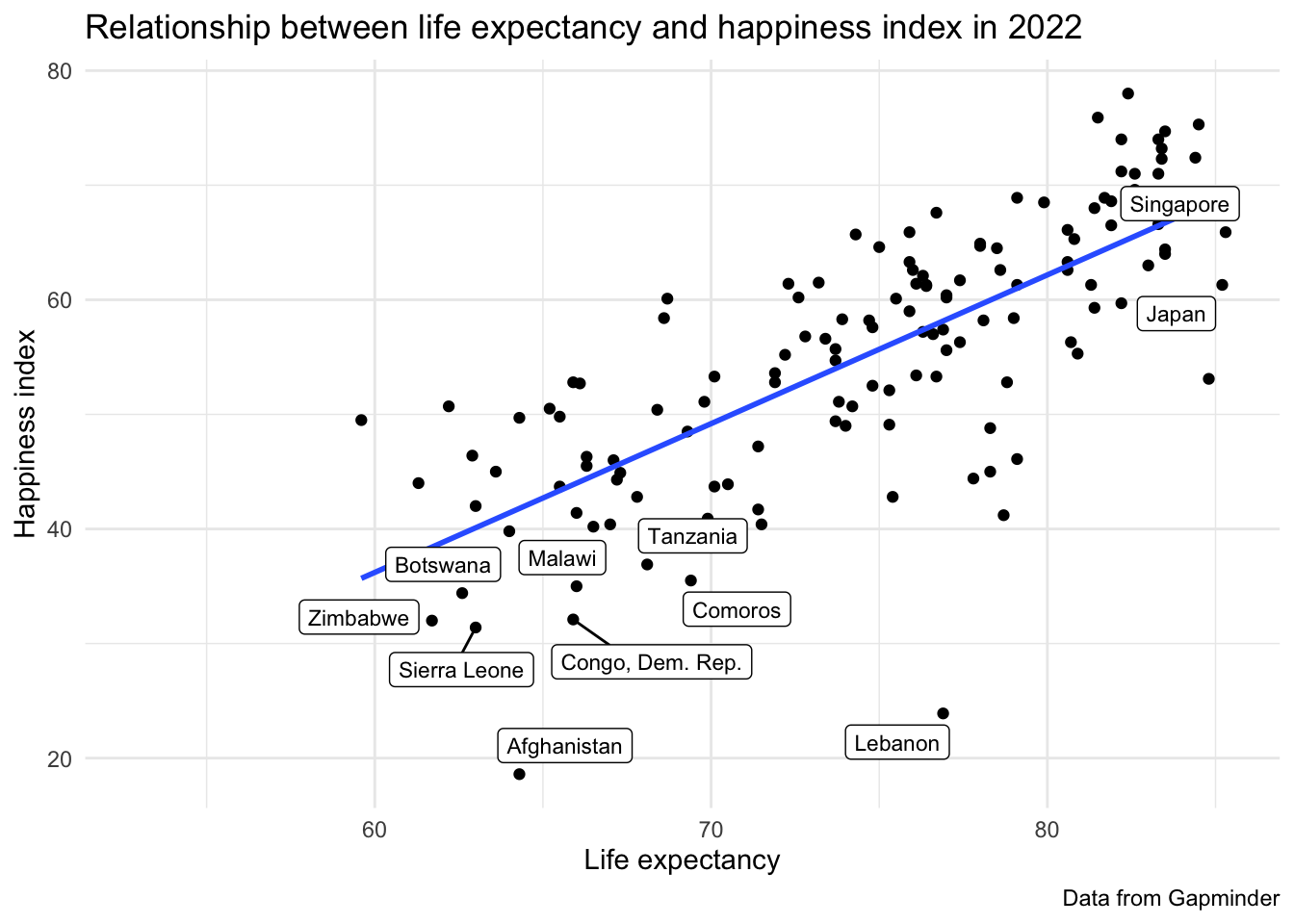
by = c("country", "year"))In this case, you want a data frame that includes only the values that are in both the life expectancy and the happiness datasets. And, we want to be able to have a column with the life expectancy and a column with the happiness value.
I am not expecting you to be able to make a plot but I wanted to just give you a sense of the kinds of things you’ll be learning in class.
# create a df with the extreme values for life exp and happiness
extremes <- for_correlation_wide |>
  filter(life_expectancy_2022 > 85 | happy_value_2022 < 38)

# create a plot
for_correlation_wide |>
  ggplot(aes(x = life_expectancy_2022, y = happy_value_2022)) +
  geom_point() +
  geom_smooth(method = "lm", se = FALSE) +
  ggrepel::geom_label_repel(data = extremes,
                            aes(x = life_expectancy_2022, y = happy_value_2022,
                                label = country),
                            size = 3) +
  theme_minimal() +
  labs(x = "Life expectancy",
       y = "Happiness index",
       title = "Relationship between life expectancy and happiness index in 2022",
       caption = "Data from Gapminder")