library(tidyverse)ggplot 101 recitation 🎃
Week 5
Introduction
We are going to practice using ggplot2 today, focusing wrangling data, mapping variables to aesthetics, and adding geoms.
We are going to use data from the TidyTuesday project. For this recitation, we are going to use the Giant Pumpkins data which is collected from the Great Pumpkin Commonwealth. You can learn more about how the data is structured here.
Today, you are going to make this plot:
Load packages
First we will load the tidyverse. The tidyverse also contains the package lubridate which you might use to help later with dates.
Read in data
You can read in the data directly from a url or you can download the file and read it in locally. To get the file locally, you can go to this link, right click on Raw, and save link as pumpkins.txt in your working directory.
# from a url
pumpkins_raw <- read_csv('https://raw.githubusercontent.com/rfordatascience/tidytuesday/master/data/2021/2021-10-19/pumpkins.csv')
Rows: 28065 Columns: 14
── Column specification ────────────────────────────────────────────────────────
Delimiter: ","
chr (14): id, place, weight_lbs, grower_name, city, state_prov, country, gpc...
ℹ Use `spec()` to retrieve the full column specification for this data.
ℹ Specify the column types or set `show_col_types = FALSE` to quiet this message.# download and read in from your computer
pumpkins_raw <- read_csv("pumpkins.txt")Wrangling
Turn one character column into two ✂️
From both looking at the data, and reading about the variable id on the documentation page, you see that it contains two type of observations. Since we want to be able to filter for only Giant Pumpkins, and we will want to plot x = year we need to separate them.
To use them separately, we need to separate this column into two columns such like year and type.
Try doing this with the function separate() or separate_wider_delim(). I will show you both ways and then just use separate() for ther rest of the example.
pumpkins_raw |>
  separate(col = id,
           into = c("year", "type"), # combine year and type as a vector
           sep = "-",
           remove = FALSE) # if you want to keep id, not required
# A tibble: 28,065 × 16
id year type place weight_lbs grower_name city state_prov country
<chr> <chr> <chr> <chr> <chr> <chr> <chr> <chr> <chr>
1 2013-F 2013 F 1 154.50 Ellenbecker, To… Glea… Wisconsin United…
2 2013-F 2013 F 2 146.50 Razo, Steve New … Ohio United…
3 2013-F 2013 F 3 145.00 Ellenbecker, To… Glen… Wisconsin United…
4 2013-F 2013 F 4 140.80 Martin, Margare… Comb… Wisconsin United…
5 2013-F 2013 F 5 139.00 Barlow, John <NA> Wisconsin United…
6 2013-F 2013 F 5 139.00 Werner, Quinn Saeg… Pennsylva… United…
7 2013-F 2013 F 7 136.50 Treece, Jef West… Oregon United…
8 2013-F 2013 F 8 136.00 Werner, Quinn Saeg… Pennsylva… United…
9 2013-F 2013 F 9 134.50 Rose, Jerry Hunt… Ohio United…
10 2013-F 2013 F 10 134.00 Coolen, Russell Bout… Nova Scot… Canada
# ℹ 28,055 more rows
# ℹ 7 more variables: gpc_site <chr>, seed_mother <chr>,
# pollinator_father <chr>, ott <chr>, est_weight <chr>, pct_chart <chr>,
# variety <chr>pumpkins_raw |>
separate_wider_delim(cols = id,
delim = "-", # delimiter is a hyphen
names = c("year", "type"), # combine year and type as a vector
cols_remove = FALSE) # to keep id, not required# A tibble: 28,065 × 16
year type id place weight_lbs grower_name city state_prov country
<chr> <chr> <chr> <chr> <chr> <chr> <chr> <chr> <chr>
1 2013 F 2013-F 1 154.50 Ellenbecker, To… Glea… Wisconsin United…
2 2013 F 2013-F 2 146.50 Razo, Steve New … Ohio United…
3 2013 F 2013-F 3 145.00 Ellenbecker, To… Glen… Wisconsin United…
4 2013 F 2013-F 4 140.80 Martin, Margare… Comb… Wisconsin United…
5 2013 F 2013-F 5 139.00 Barlow, John <NA> Wisconsin United…
6 2013 F 2013-F 5 139.00 Werner, Quinn Saeg… Pennsylva… United…
7 2013 F 2013-F 7 136.50 Treece, Jef West… Oregon United…
8 2013 F 2013-F 8 136.00 Werner, Quinn Saeg… Pennsylva… United…
9 2013 F 2013-F 9 134.50 Rose, Jerry Hunt… Ohio United…
10 2013 F 2013-F 10 134.00 Coolen, Russell Bout… Nova Scot… Canada
# ℹ 28,055 more rows
# ℹ 7 more variables: gpc_site <chr>, seed_mother <chr>,
# pollinator_father <chr>, ott <chr>, est_weight <chr>, pct_chart <chr>,
# variety <chr>Select observations by their values 🎃
Now that you separated id into year and type we want to keep only the data for Giant Pumpkins, and only for the first place pumpkins..
pumpkins_raw |>
  separate(col = id,
           into = c("year", "type"), # combine year and type as a vector
           sep = "-",
           remove = FALSE) |>  # if you want to keep id, not required
  filter(type == "P" & place == "1") # only type P AND first place
# A tibble: 9 × 16
id year type place weight_lbs grower_name city state_prov country
<chr> <chr> <chr> <chr> <chr> <chr> <chr> <chr> <chr>
1 2013-P 2013 P 1 2,032.00 Mathison, Tim Napa California United…
2 2014-P 2014 P 1 2,323.70 Meier, Beni Pfun… Other Switze…
3 2015-P 2015 P 1 2,230.50 Wallace, Ron Gree… Rhode Isl… United…
4 2016-P 2016 P 1 2,624.60 Willemijns, Math… Deur… East Flan… Belgium
5 2017-P 2017 P 1 2,363.00 Holland, Joel Sumn… Washington United…
6 2018-P 2018 P 1 2,528.00 Geddes, Steve Bosc… New Hamps… United…
7 2019-P 2019 P 1 2,517.00 Haist, Karl & Be… Clar… New York United…
8 2020-P 2020 P 1 2,593.70 Paton, Ian & Stu… Ever… England United…
9 2021-P 2021 P 1 2,702.90 Cutrupi, Stefano Radd… Tuscany Italy
# ℹ 7 more variables: gpc_site <chr>, seed_mother <chr>,
# pollinator_father <chr>, ott <chr>, est_weight <chr>, pct_chart <chr>,
# variety <chr>Remove pesky strings 😑
Let’s see what plotting would look like now:
pumpkins_raw |>
  separate(col = id,
           into = c("year", "type"), # combine year and type as a vector
           sep = "-",
           remove = FALSE) |>  # if you want to keep id, not required
  filter(type == "P" & place == "1") |>  # only type P AND first place
  ggplot(aes(x = year, y = weight_lbs)) +
    geom_point()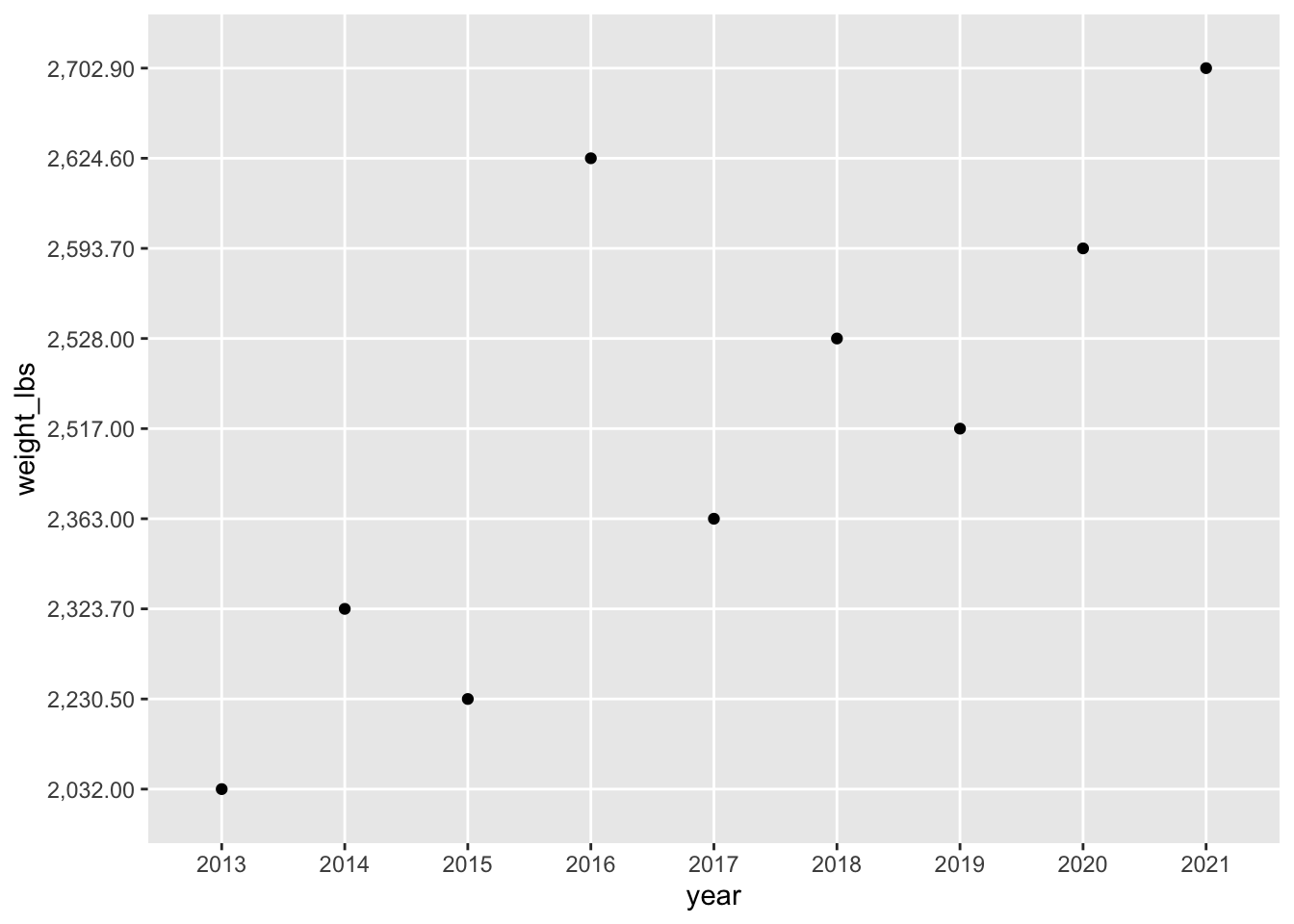
If we try and make a line plot it just simply gives us no plot.
pumpkins_raw |>
  separate(col = id,
           into = c("year", "type"), # combine year and type as a vector
           sep = "-",
           remove = FALSE) |>  # if you want to keep id, not required
  filter(type == "P" & place == "1") |>  # only type P AND first place
  ggplot(aes(x = year, y = weight_lbs)) +
    geom_line()
`geom_line()`: Each group consists of only one observation.
ℹ Do you need to adjust the group aesthetic?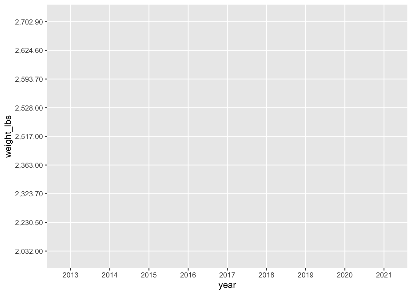
If we look at our data, we see that both year and weight_lbs are actually character strings and weight_lbs has a comma that is preventing R from viewing it as a number. To plot them to x and y, they need to be numeric so let’s fix that.
If we simply just trying and convert weight_lbs to be numeric using as.numeric() this does not work. We just end up with a column on NAs. Wow this comma gets in the way!
# doesn't convert weight_lbs to numeric
pumpkins_raw |>
  separate(col = id,
           into = c("year", "type"), # combine year and type as a vector
           sep = "-",
           remove = FALSE) |>  # if you want to keep id, not required
  filter(type == "P" & place == "1") |>  # only type P AND first place
  mutate(weight_lbs = as.numeric(weight_lbs))
Warning: There was 1 warning in `mutate()`.
ℹ In argument: `weight_lbs = as.numeric(weight_lbs)`.
Caused by warning:
! NAs introduced by coercion# A tibble: 9 × 16
id year type place weight_lbs grower_name city state_prov country
<chr> <chr> <chr> <chr> <dbl> <chr> <chr> <chr> <chr>
1 2013-P 2013 P 1 NA Mathison, Tim Napa California United…
2 2014-P 2014 P 1 NA Meier, Beni Pfun… Other Switze…
3 2015-P 2015 P 1 NA Wallace, Ron Gree… Rhode Isl… United…
4 2016-P 2016 P 1 NA Willemijns, Math… Deur… East Flan… Belgium
5 2017-P 2017 P 1 NA Holland, Joel Sumn… Washington United…
6 2018-P 2018 P 1 NA Geddes, Steve Bosc… New Hamps… United…
7 2019-P 2019 P 1 NA Haist, Karl & Be… Clar… New York United…
8 2020-P 2020 P 1 NA Paton, Ian & Stu… Ever… England United…
9 2021-P 2021 P 1 NA Cutrupi, Stefano Radd… Tuscany Italy
# ℹ 7 more variables: gpc_site <chr>, seed_mother <chr>,
# pollinator_father <chr>, ott <chr>, est_weight <chr>, pct_chart <chr>,
# variety <chr>We can remove the comma by using the function str_remove() nested within a mutate() call to actually change the column. Remember, we don’t want to just remove the thousands place comma in one number, we want to edit the dataset to remove the comma.
pumpkins_raw |>
  separate(col = id,
           into = c("year", "type"), # combine year and type as a vector
           sep = "-",
           remove = FALSE) |>  # if you want to keep id, not required
  filter(type == "P" & place == "1") |>  # only type P AND first place
  mutate(weight_lbs = str_remove(weight_lbs, ",")) # remove comma
# A tibble: 9 × 16
id year type place weight_lbs grower_name city state_prov country
<chr> <chr> <chr> <chr> <chr> <chr> <chr> <chr> <chr>
1 2013-P 2013 P 1 2032.00 Mathison, Tim Napa California United…
2 2014-P 2014 P 1 2323.70 Meier, Beni Pfun… Other Switze…
3 2015-P 2015 P 1 2230.50 Wallace, Ron Gree… Rhode Isl… United…
4 2016-P 2016 P 1 2624.60 Willemijns, Math… Deur… East Flan… Belgium
5 2017-P 2017 P 1 2363.00 Holland, Joel Sumn… Washington United…
6 2018-P 2018 P 1 2528.00 Geddes, Steve Bosc… New Hamps… United…
7 2019-P 2019 P 1 2517.00 Haist, Karl & Be… Clar… New York United…
8 2020-P 2020 P 1 2593.70 Paton, Ian & Stu… Ever… England United…
9 2021-P 2021 P 1 2702.90 Cutrupi, Stefano Radd… Tuscany Italy
# ℹ 7 more variables: gpc_site <chr>, seed_mother <chr>,
# pollinator_father <chr>, ott <chr>, est_weight <chr>, pct_chart <chr>,
# variety <chr>Commas, gone! 👏👏👏
Convert character to numeric 🔢
Now the comma is gone, you can simply change the variable weight_lbs from a character to numeric, so it can be plotted like a number. To change the column type, we are going to use the as.numeric() function. Here’s some example about how to use as.numeric().
Let’s add this to our growing pipe.
pumpkins_raw |>
  separate(col = id,
           into = c("year", "type"), # combine year and type as a vector
           sep = "-",
           remove = FALSE) |>  # if you want to keep id, not required
  filter(type == "P" & place == "1") |>  # only type P AND first place
  mutate(weight_lbs = str_remove(weight_lbs, ",")) |> # remove comma
  mutate(weight_lbs = as.numeric(weight_lbs)) # convert weight_lbs to numeric
# A tibble: 9 × 16
id year type place weight_lbs grower_name city state_prov country
<chr> <chr> <chr> <chr> <dbl> <chr> <chr> <chr> <chr>
1 2013-P 2013 P 1 2032 Mathison, Tim Napa California United…
2 2014-P 2014 P 1 2324. Meier, Beni Pfun… Other Switze…
3 2015-P 2015 P 1 2230. Wallace, Ron Gree… Rhode Isl… United…
4 2016-P 2016 P 1 2625. Willemijns, Math… Deur… East Flan… Belgium
5 2017-P 2017 P 1 2363 Holland, Joel Sumn… Washington United…
6 2018-P 2018 P 1 2528 Geddes, Steve Bosc… New Hamps… United…
7 2019-P 2019 P 1 2517 Haist, Karl & Be… Clar… New York United…
8 2020-P 2020 P 1 2594. Paton, Ian & Stu… Ever… England United…
9 2021-P 2021 P 1 2703. Cutrupi, Stefano Radd… Tuscany Italy
# ℹ 7 more variables: gpc_site <chr>, seed_mother <chr>,
# pollinator_father <chr>, ott <chr>, est_weight <chr>, pct_chart <chr>,
# variety <chr>Plot
With the weight_lbs variable corrected, we can re-plot.
pumpkins_raw |>
  separate(col = id,
           into = c("year", "type"), # combine year and type as a vector
           sep = "-",
           remove = FALSE) |>  # if you want to keep id, not required
  filter(type == "P" & place == "1") |>  # only type P AND first place
  mutate(weight_lbs = str_remove(weight_lbs, ",")) |> # remove comma
  mutate(weight_lbs = as.numeric(weight_lbs)) |> # convert weight_lbs to numeric
  ggplot(aes(x = year, y = weight_lbs)) + # map year to x, weight_lbs to y in aes()
    geom_point() + # add points
    geom_line() # add lines
`geom_line()`: Each group consists of only one observation.
ℹ Do you need to adjust the group aesthetic?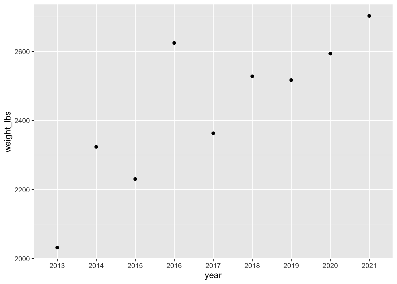
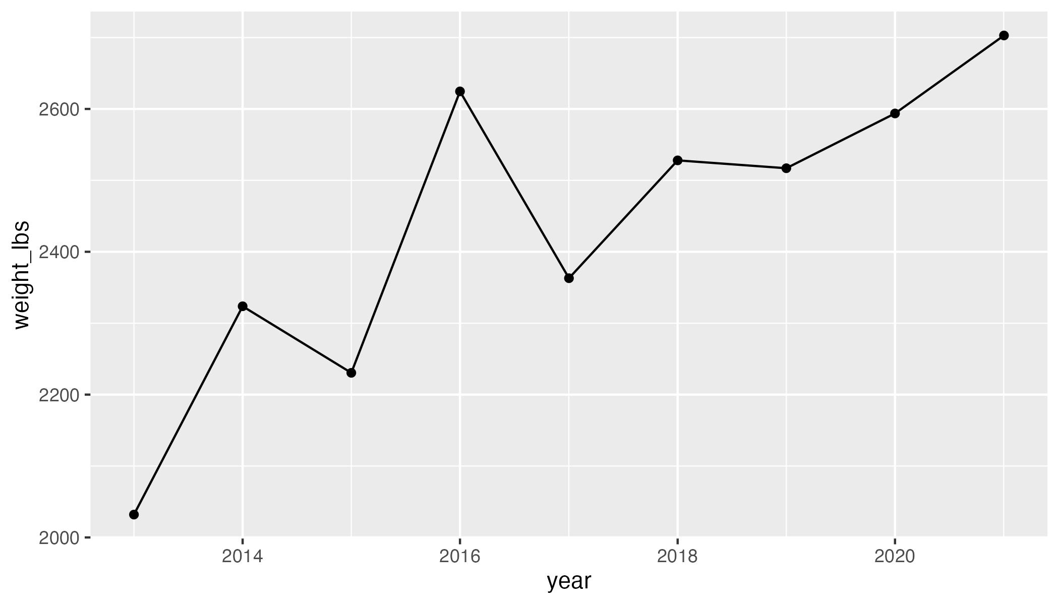
Convert year to numeric or a date
The lines aren’t showing up because year is a character variable. We can change year to be either a number or a date.
Converting year to numeric.
pumpkins_raw |>
  separate(col = id,
           into = c("year", "type"), # combine year and type as a vector
           sep = "-",
           remove = FALSE) |>  # if you want to keep id, not required
  filter(type == "P" & place == "1") |>  # only type P AND first place
  mutate(weight_lbs = str_remove(weight_lbs, ",")) |> # remove comma
  mutate(weight_lbs = as.numeric(weight_lbs)) |> # convert weight_lbs to numeric
  mutate(year = as.numeric(year)) |> # convert year to numeric
  ggplot(aes(x = year, y = weight_lbs)) + # map year to x, weight_lbs to y in aes()
    geom_point() + # add points
    geom_line() # add lines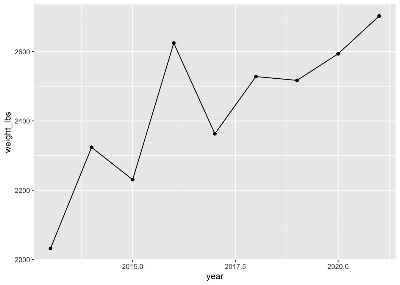
This creates some issues with the x-axis tick labels - since 2017.5 isn’t a meaningful year. You can change that with scale_*() by setting the axis breaks but we haven’t learned how to do that yet.
# scale_x_continous lets you scale how year is mapped to x
# seq gives you a sequence, here from 2013 to 2021, by 2s
pumpkins_raw |>
  separate(col = id,
           into = c("year", "type"), # combine year and type as a vector
           sep = "-",
           remove = FALSE) |>  # if you want to keep id, not required
  filter(type == "P" & place == "1") |>  # only type P AND first place
  mutate(weight_lbs = str_remove(weight_lbs, ",")) |> # remove comma
  mutate(weight_lbs = as.numeric(weight_lbs)) |> # convert weight_lbs to numeric
  mutate(year = as.numeric(year)) |> # convert year to numeric
  ggplot(aes(x = year, y = weight_lbs)) + # map year to x, weight_lbs to y in aes()
    geom_point() + # add points
    geom_line() + # add lines
    scale_x_continuous(breaks = seq(2013, 2021, 2)) # adjust x-axis breaks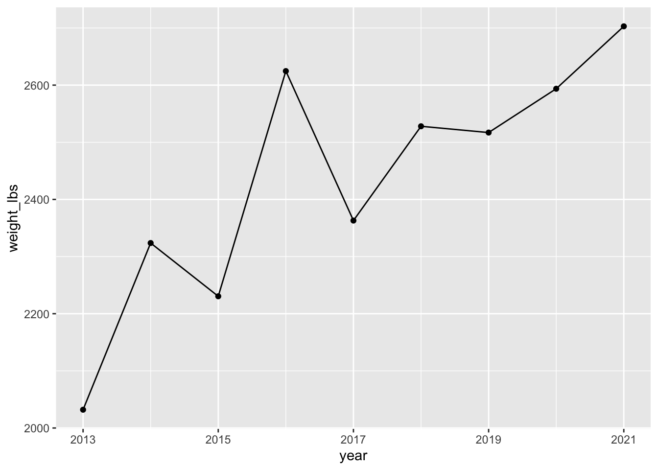
Can convert to date using as.Date() with some arguments.
pumpkins_raw |>
  separate(col = id,
           into = c("year", "type"), # combine year and type as a vector
           sep = "-",
           remove = FALSE) |>  # if you want to keep id, not required
  filter(type == "P" & place == "1") |>  # only type P AND first place
  mutate(weight_lbs = str_remove(weight_lbs, ",")) |> # remove comma
  mutate(weight_lbs = as.numeric(weight_lbs)) |> # convert weight_lbs to numeric
  mutate(year = as.Date(year, "%Y")) |> # convert to date in format year
  ggplot(aes(x = year, y = weight_lbs)) + # map year to x, weight_lbs to y in aes()
    geom_point() + # add points
    geom_line()  # add lines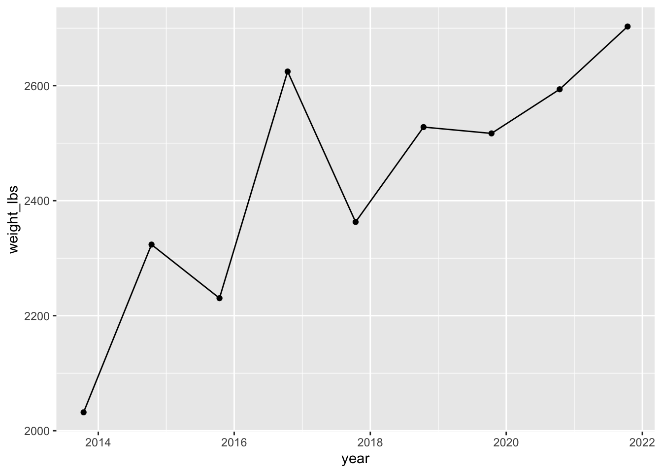
You can also convert year to be a date using functions from the package lubridate and the function ymd().
# ymd() converts characters to dates
pumpkins_raw |>
  separate(col = id,
           into = c("year", "type"), # combine year and type as a vector
           sep = "-",
           remove = FALSE) |>  # if you want to keep id, not required
  filter(type == "P" & place == "1") |>  # only type P AND first place
  mutate(weight_lbs = str_remove(weight_lbs, ",")) |> # remove comma
  mutate(weight_lbs = as.numeric(weight_lbs)) |> # convert weight_lbs to numeric
  mutate(year = ymd(year, truncated = 2L)) |> # truncated allows for incomplete dates
  ggplot(aes(year, weight_lbs)) +
    geom_point() +
    geom_line()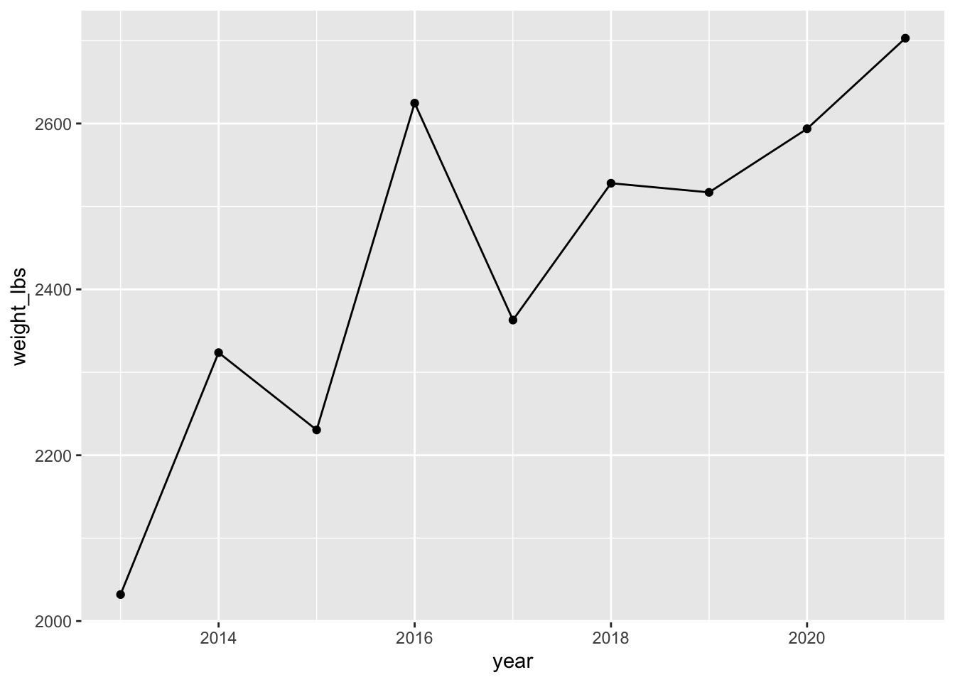
Playing around
Other plot types
Try using different geoms besides geom_point() and geom_line(). Which ones might make sense in this situation?
A bar chart. Note that you can pass color also as hex codes and R is smart enough to highlight those colors with that color if you use RStudio and RMarkdown/Quarto.
pumpkins_raw |>
  separate(col = id,
           into = c("year", "type"), # combine year and type as a vector
           sep = "-",
           remove = FALSE) |>  # if you want to keep id, not required
  filter(type == "P" & place == "1") |>  # only type P AND first place
  mutate(weight_lbs = str_remove(weight_lbs, ",")) |> # remove comma
  mutate(weight_lbs = as.numeric(weight_lbs)) |> # convert weight_lbs to numeric
  mutate(year = as.Date(year, "%Y")) |> # convert to date in format year
  ggplot(aes(x = year, y = weight_lbs)) + # map year to x, weight_lbs to y in aes()
    geom_col(color = "black", fill = "#d36e0e")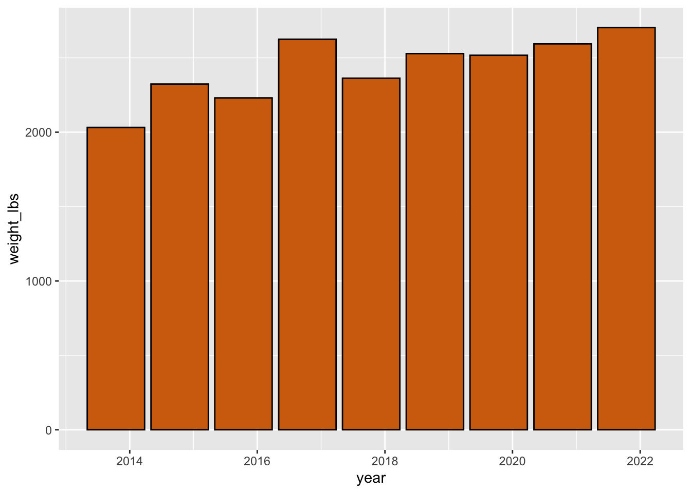
A lollypop chart. shape = 21 is my favorite shape, its the circle where you can control the color the outline with color and the color of the inside with fill.
pumpkins_raw |>
  separate(col = id,
           into = c("year", "type"), # combine year and type as a vector
           sep = "-",
           remove = FALSE) |>  # if you want to keep id, not required
  filter(type == "P" & place == "1") |>  # only type P AND first place
  mutate(weight_lbs = str_remove(weight_lbs, ",")) |> # remove comma
  mutate(weight_lbs = as.numeric(weight_lbs)) |> # convert weight_lbs to numeric
  mutate(year = as.Date(year, "%Y")) |> # convert to date in format year
  ggplot(aes(x = year, y = weight_lbs)) + # map year to x, weight_lbs to y in aes()
    geom_segment(aes(x = year, xend = year, y = 0, yend = weight_lbs)) + # create lines
    geom_point(fill = "#d36e0e", color = "black", size = 3, shape = 21)  # add points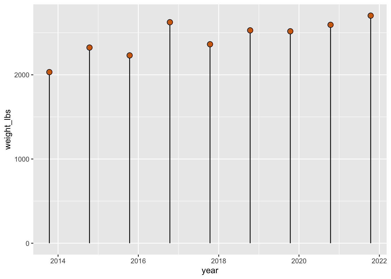
Blue lines
Can you color all the lines blue?
pumpkins_raw |>
  separate(col = id,
           into = c("year", "type"), # combine year and type as a vector
           sep = "-",
           remove = FALSE) |>  # if you want to keep id, not required
  filter(type == "P" & place == "1") |>  # only type P AND first place
  mutate(weight_lbs = str_remove(weight_lbs, ",")) |> # remove comma
  mutate(weight_lbs = as.numeric(weight_lbs)) |> # convert weight_lbs to numeric
  mutate(year = as.Date(year, "%Y")) |> # convert to date in format year
  ggplot(aes(x = year, y = weight_lbs)) + # map year to x, weight_lbs to y in aes()
    geom_point() + # points stay default
    geom_line(color = "blue") # lines blue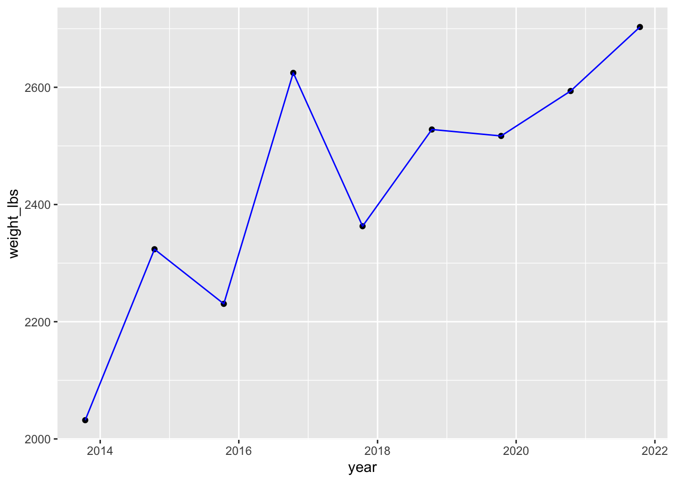
Color by year
Can you color the data based on year?
If you color a continuous variable by color, you will get a continuous color scale.
pumpkins_raw |>
  separate(col = id,
           into = c("year", "type"), # combine year and type as a vector
           sep = "-",
           remove = FALSE) |>  # if you want to keep id, not required
  filter(type == "P" & place == "1") |>  # only type P AND first place
  mutate(weight_lbs = str_remove(weight_lbs, ",")) |> # remove comma
  mutate(weight_lbs = as.numeric(weight_lbs)) |> # convert weight_lbs to numeric
  mutate(year = as.Date(year, "%Y")) |> # convert to date in format year
  ggplot(aes(x = year, y = weight_lbs)) + # map year to x, weight_lbs to y in aes()
    geom_point(aes(fill = year), shape = 21) + # color points by year
    geom_line()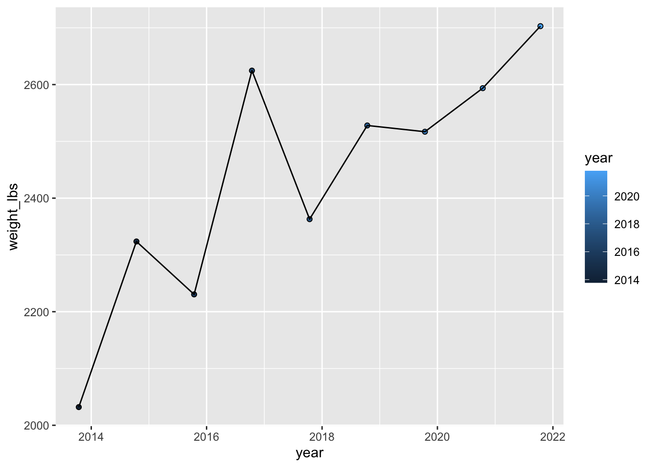
If you want that color scale to be discrete, you can either convert year to a factor in your dataset, or just convert it to a factor for your plot.
pumpkins_raw |>
  separate(col = id,
           into = c("year", "type"), # combine year and type as a vector
           sep = "-",
           remove = FALSE) |>  # if you want to keep id, not required
  filter(type == "P" & place == "1") |>  # only type P AND first place
  mutate(weight_lbs = str_remove(weight_lbs, ",")) |> # remove comma
  mutate(weight_lbs = as.numeric(weight_lbs)) |> # convert weight_lbs to numeric
  mutate(year = as.Date(year, "%Y")) |> # convert to date in format year
  ggplot(aes(x = year, y = weight_lbs)) + # map year to x, weight_lbs to y in aes()
    geom_point(aes(fill = as.factor(year)), shape = 21) + # year as factor for discrete colors
    geom_line()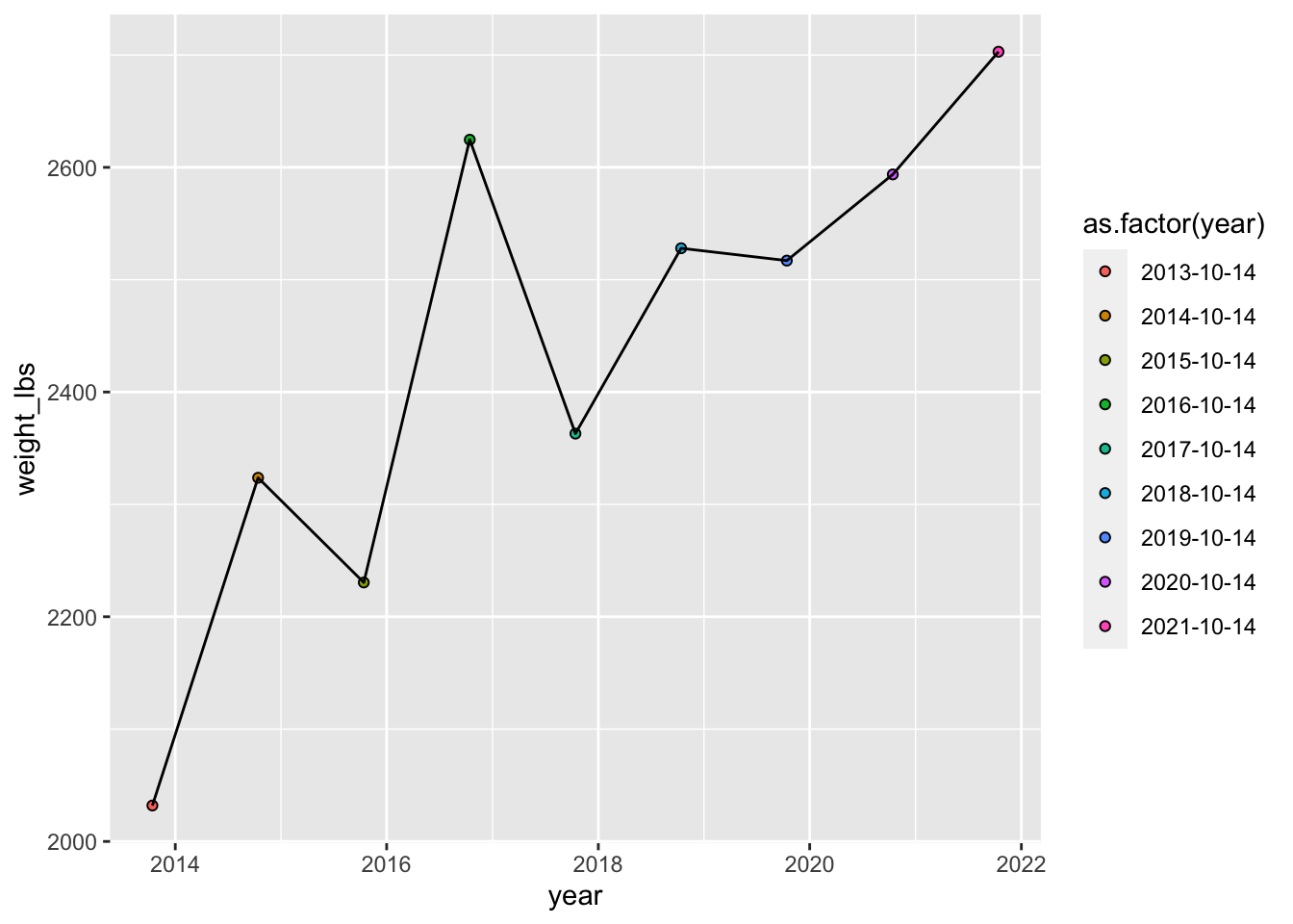
Color and shape by country
Can you change color and change shape based on country?
pumpkins_raw |>
  separate(col = id,
           into = c("year", "type"), # combine year and type as a vector
           sep = "-",
           remove = FALSE) |>  # if you want to keep id, not required
  filter(type == "P" & place == "1") |>  # only type P AND first place
  mutate(weight_lbs = str_remove(weight_lbs, ",")) |> # remove comma
  mutate(weight_lbs = as.numeric(weight_lbs)) |> # convert weight_lbs to numeric
  mutate(year = as.Date(year, "%Y")) |> # convert to date in format year
  ggplot(aes(x = year, y = weight_lbs)) + # map year to x, weight_lbs to y in aes()
    geom_point(aes(color = as.factor(country), shape = country), size = 3) + # year as factor for discrete colors
    geom_line()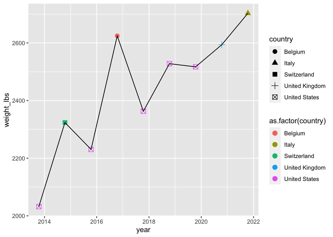
Distribution of all giant pumpkins in 2021
Can you make a plot showing the distribution of weights of all giant pumpkins entered in 2021?
pumpkins_raw |>
  separate(col = id,
           into = c("year", "type"), # combine year and type as a vector
           sep = "-",
           remove = FALSE) |>  # if you want to keep id, not required
  filter(type == "P") |>  # only type P
  filter(year == 2021) |> # only pumpkins from 2021
  mutate(weight_lbs = str_remove(weight_lbs, ",")) |> # remove comma
  mutate(weight_lbs = as.numeric(weight_lbs)) |> # convert weight_lbs to numeric
  mutate(year = as.Date(year, "%Y")) |> # convert to date in format year
  ggplot(aes(x =  weight_lbs)) + # map weight_lbs to x within aes()
    geom_density()
Warning: There was 1 warning in `mutate()`.
ℹ In argument: `weight_lbs = as.numeric(weight_lbs)`.
Caused by warning:
! NAs introduced by coercionWarning: Removed 1 rows containing non-finite values (`stat_density()`).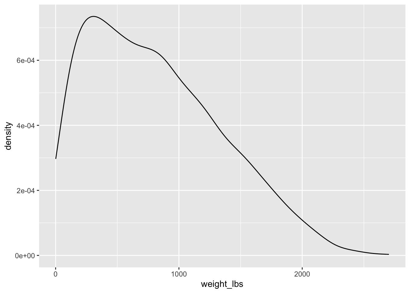
Could also do a histogram instead.
pumpkins_raw |>
  separate(col = id,
           into = c("year", "type"), # combine year and type as a vector
           sep = "-",
           remove = FALSE) |>  # if you want to keep id, not required
  filter(type == "P") |>  # only type P
  filter(year == 2021) |> # only pumpkins from 2021
  mutate(weight_lbs = str_remove(weight_lbs, ",")) |> # remove comma
  mutate(weight_lbs = as.numeric(weight_lbs)) |> # convert weight_lbs to numeric
  mutate(year = as.Date(year, "%Y")) |> # convert to date in format year
  ggplot(aes(x =  weight_lbs)) + # map weight_lbs to x within aes()
    geom_histogram(color = "black", fill = "orange") # can set number of bins or binwidth too
Warning: There was 1 warning in `mutate()`.
ℹ In argument: `weight_lbs = as.numeric(weight_lbs)`.
Caused by warning:
! NAs introduced by coercion`stat_bin()` using `bins = 30`. Pick better value with `binwidth`.Warning: Removed 1 rows containing non-finite values (`stat_bin()`).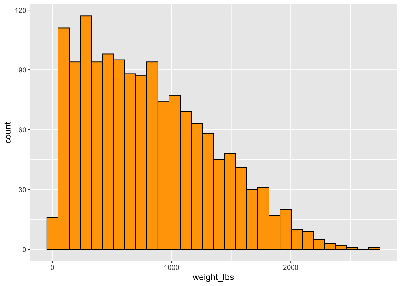
Boxplot of weights for all years
Can you make a boxplot showing the distribution of weights of all giant pumpkins across all years? Also can you add all the datapoints on top of the boxplot? Is this a good idea? Might there be a better geom to use than a boxplot?
Note that we are removed the filtering for only first place pumpkins.
pumpkins_raw |>
  separate(col = id,
           into = c("year", "type"), # combine year and type as a vector
           sep = "-",
           remove = FALSE) |>  # if you want to keep id, not required
  filter(type == "P" ) |>  # only type P - but all pumpkins now
  mutate(weight_lbs = str_remove(weight_lbs, ",")) |> # remove comma
  mutate(weight_lbs = as.numeric(weight_lbs)) |> # convert weight_lbs to numeric
  mutate(year = as.Date(year, "%Y")) |> # convert to date in format year
  ggplot(aes(x =  year, y = weight_lbs, group = year)) + # group = year to boxplot by year
    geom_boxplot(outlier.shape = NA) + # don't plot outliers on boxplot layer
    geom_jitter(alpha = 0.1) # lighten points to avoid overplotting
Warning: There was 1 warning in `mutate()`.
ℹ In argument: `weight_lbs = as.numeric(weight_lbs)`.
Caused by warning:
! NAs introduced by coercionWarning: Removed 9 rows containing non-finite values (`stat_boxplot()`).Warning: Removed 9 rows containing missing values (`geom_point()`).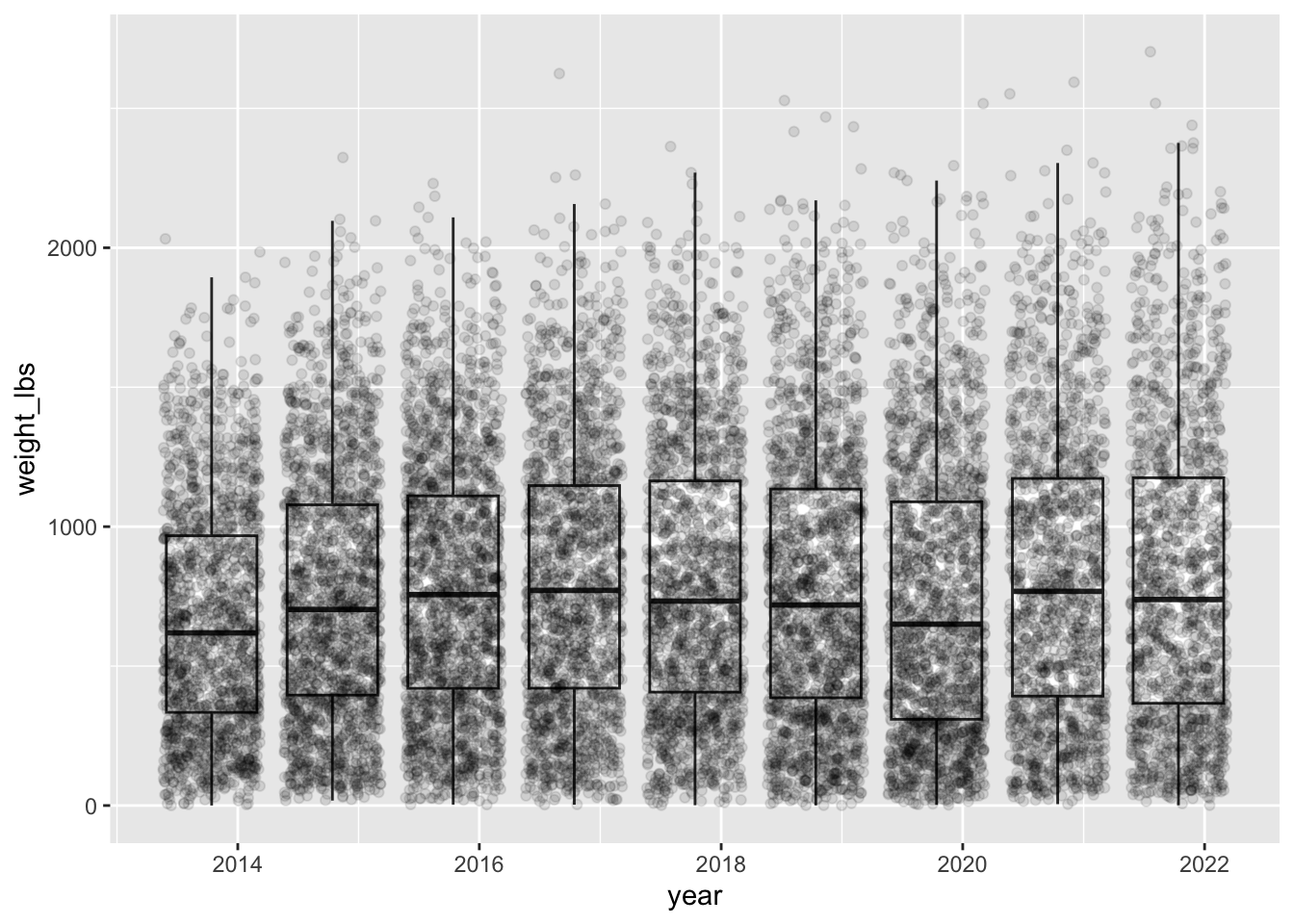
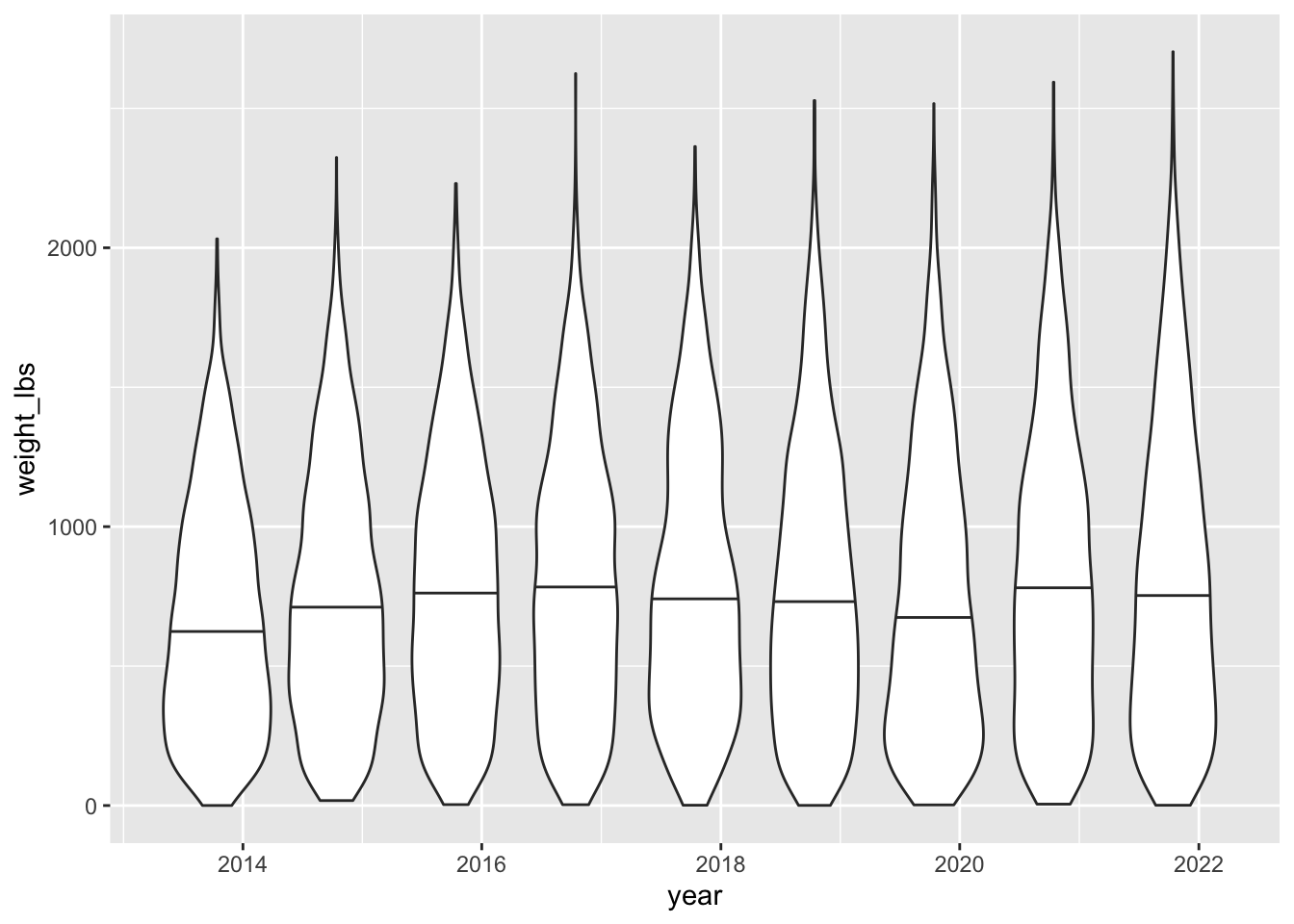
A violin plot instead.
pumpkins_raw |>
  separate(col = id,
           into = c("year", "type"), # combine year and type as a vector
           sep = "-",
           remove = FALSE) |>  # if you want to keep id, not required
  filter(type == "P" ) |>  # only type P - but all pumpkins now
  mutate(weight_lbs = str_remove(weight_lbs, ",")) |> # remove comma
  mutate(weight_lbs = as.numeric(weight_lbs)) |> # convert weight_lbs to numeric
  mutate(year = as.Date(year, "%Y")) |> # convert to date in format year
  ggplot(aes(x =  year, y = weight_lbs, group = year)) + # group = year to boxplot by year
    geom_violin(draw_quantiles = 0.5) # violin plot showing the median
Warning: There was 1 warning in `mutate()`.
ℹ In argument: `weight_lbs = as.numeric(weight_lbs)`.
Caused by warning:
! NAs introduced by coercionWarning: Removed 9 rows containing non-finite values (`stat_ydensity()`).